
The Chelsea Surveying Ethos - John Stevens
Part one - discussion of techniques used
The Accuracy of GPS Receivers and an Attempt at
Do-It-Yourself Differential GPS - Bob Thrun
Does DIY differential GPS work, and how long do you
have to stand in one place to get good accuracy?
The field meet will have happened by the time you read this issue, but this is being written before said meet. So the report of what happened will have to be in the next issue. It looks like there will be a reasonable attendance of surveyors, and I hope to have interesting developments to report.
This is the first issue of CP for which I have more material than will fit in it. Thank you to all those who have written and are writing. Your articles will appear in due course, and CP will expand if the flow of material remains high. It looks like the surveying group is taking off!
At the moment, those members who receive Compass Points but who do not subscribe to the Journal are mailed with a copy of the Newssheet. From the next issue of CP we will not do this. Instead, any important 'secretarial' information will be duplicated in CP. Anyone who specifically wants a copy of the newssheet in addition to CP can ask for one, and we will mail it at no additional charge.
As you know, the BCRA Cave Surveying Group (CSG) has existed 'unofficially' for some time now, as part of the Cave Radio & Electronics Group. This saves the duplication of resources (printing, membership list, info sheets, accounts mailing). One problem with the current arrangement is, however, that the Surveying Group is not able to publicise itself to its best advantage. Not all cave surveyors realise that it exists. CREG has begun to refer to the cave surveyors as the "cave surveying group", but this is not entirely satisfactory. We are therefore trying to finalise plans to "float" a genuine CSG at our AGM, later in the year, complete with officers and constitution, although we will probably continue to act as a "secretariat" and publishing agent for the CSG. This does mean that we need at least one, and preferably two volunteers to help run the Group. Under the existing arrangements you will have very little actual work to do, but as the CSG grows, then we may have to do our share of the CREG/CSG work. Please consider whether you would be interested and could give up a couple of hours a quarter for keeping a membership list, sending out info sheets to enquirers, or stuffing envelopes.
Compass & Tape (The US Cave Surveying magazine) issues 38 and 39 have both appeared since my last roundup in CP 9, but due to lack of space this issue, only issue 38 is reviewed here:
Editorial comment from chairman. The converging effects of the NSS Map Salon competition and computers over the last 10 years.
LRCFs: we can do better. Peter Sprouse arguing that recording Left-Right-Ceiling-Floor info is a poor technique in comparison to drawing cross-sections.
The art of Lead Tape and other related ramblings. Long article by Tom Moss abou the various aspects of being 'lead tape' - picking stations, marking stations, lighting stations, reading the tape, measuring passage dimensions, checking leads, and communicating.
Observations on Survey Sketch Quality. Three experienced surveyors give their opinions on a selection of actual survey sketches ranbging from the awful to the excellent.
Creating Electronic Maps from True to Scale Cave Survey Sketches. Garry Petrie talks about ways of scanning in sketches, converting the results to vector files and using them in your final survey.
On Guidelines for Electronic Maps. Start of discussion on how to judge 'electronic' as opposed to paper maps at the NSS convention Map Salon.
Survey Standards for Hidden River Cave Project
Graphical Solution for Determining Ceiling Heights
Survex version 0.69b2 has been released on the net for people to experiment with. This is test release, and we haven't finished docs to go with the new features yet, but email <wookey@aleph1.co.uk>, if you want a copy to play with. Once it is believed stable we will be shipping copies to existing members of the user group, and anyone else who asks.
Survex 0.69b2
General:
Caverot:
Printer Drivers:
Survex:
Survex 0.61 & 0.62 were releases with only slight changes:
Survex 0.62
Survex 0.61
Dear Wookey,
I gather you chatted to my colleague Andrew Chamberlain at the Cave Science symposium in Stafford and were interested in hearing about the ultrasonic cave scanning I've been working on. It's an extension of a fairly old idea about using ultrasonic transducers for robot/computer vision and obstacle avoidance with a directional ultrasound transmitter and receiver mounted on a stepper motor and various bits of electronics to send an receive an ultrasound pulse. This all gets stored on a laptop PC using the printer port for data capture. You end up with plots that look rather like radar scans, and these all get assembled in a CAD package to produce a 3D model of the cave.
The results are quite pleasing considering the whole thing cost less than 100 pounds to build, but I'm hoping to get some rather more serious money to do it properly - the whole thing is rather time consuming, but could be automated. The main limitation is actually the beam spread on the ultrasound transducers which smears the data and limits the passage diameter I can work with.
One day, in the not too dim and distant future, I shall get around to writing this up properly which may interest you. I'd also be interested in contacting anyone who might be able to help improving the design.
Bill Sellers
----
Dr. Bill Sellers, Email: bill.sellers@ed.ac.uk
Department of Anatomy, The University of Edinburgh,
John Stevens
You would be hard pressed to have avoided hearing all about the huge task that has been going on in surveying Ogof Draenen as it has been discovered. The surveying has happened in two largely independent stages. The explorers have done a rough & ready survey as they went along, and Chelsea Speleological Society are doing a proper grade 5 survey for publication. Here is the first of two articles which details the methods used by those surveyors, and the reasoning behind them. Future issues will have the second part of this article, as well as a detailed account of the actual surveying by those involved.
Part 1
I am not sure where to start so much of this first
section can be found in the BCRA booklet "Introduction to
Cave Surveying". This is what it has to say about grade 5
surveying. First the centreline of the survey,
"Grade 5 :- A magnetic survey. Horizontal and vertical angles accurate to +-1 degree. Distance accurate to +-10cm. Station position error less than 10cm."
This is the statement in the normal table most people look at but frequently they fail to take full heed of the notes that go with the table. These state :-
"1. The above table ... intended only as an aide memoir....must be read in conjunction with the comments below.
2. In all cases it is necessary to follow the spirit of the definition and not just the letter.
4. Accuracy means the nearness of a result to the true value. It must not be confused with precision which is the nearness of a number of repeat results to each other, irrespective of their accuracy.
6. It is essential for instrument to be properly calibrated to attain grade 5.
7. A grade 6 survey requires the compass to be used at the limit of possible accuracy, i.e. accurate to +-0.5 degrees. Clinometer readings to be to the same accuracy. Distance and station position error must be accurate to at least +-2.5cm and will require the use of tripods or similar techniques."
Other comments that are also made and must be born in mind are :-
"It is important when assigning a grade to a survey to give the one actually attained and not what it had originally been intended to attain - they may not be the same."
Because numbers have been given in the table I have seen people use these as the precision to take the reading. They have also been used by some programmers to set the "grade 5 standard deviations" in their surveying programs. The real question is what precision do we need to use to achieve the required accuracy to attain a grade 5 survey under normal conditions? By examples later in the BCRA booklet, some of these questions are answered.
The easiest way to visualise how accurate a survey
is to look at a closed loop. What affects each station in that
loop and how much can we allow each successive station to move
from its position defined by it adjacent legs. It's position has
the following errors :- station position, tape error, compass
error, clino error. The sum of all these error should be less
than 10cm on the maximum error leg. To understand this we have
to go through each of the four contributing errors and see how
we can reduce them so that a high grade can be achieved.
"- is the maximum distance between any of the points to which and from which the various measurements were made at the station." In layman's terms, how much you moved the station between the various readings. To reduce this error to 1-2cm as a max. we always use fixed stations. i.e. wall, stone on the floor, box or BDH if it's not an instrument station (see later). The station can then be marked by a small triangle or cross (1cm across is more than enough, any larger can start increasing the error again and can be an eyesore). A cap light (off the helmet so they can see what they are doing) or smaller light can then be used to put on the station or adjacent to it on the wall. The reading of compass and clino are then taken to the light, it's reverse position on the next leg will then be only millimetres different.
Hint :- we use the claw end of the tape measure for
the instrument reader and have attached a nail on a short string
to the reel end of the tape so the tape man can also neatly and
accurately mark his station. It stops him look for a scratching
stone or carrying one around with him, which has also been known.
As we use fixed stations the tape can be pulled taut and read to the nearest 1cm. (Having the tape taut can make 2-3cm difference.) We also throw away a broken tape and not try and read one with a few cms missing. This is because it is hard to keep taut and can confuse the recording of the lengths. If a tape does break on a trip then tie a knot just short of a whole metre mark and use the knot to help hold it taut. The distances should then be recorded at they appear on the tape and not adjusted. A simple note in the book saying take x metres off from leg y to z is then adequate.
We also try and keep the maximum leg length to 20m preferring a bit less if convenient. The reason for this is given in the compass error section.
The main error is normally caused by lack of calibration. We have arranged a convenient surface leg to calibrate each instrument reader and the respective instrument. This reading is taken at the start of every survey trip. It is important that they use the same method of reading for the calibration as they do for the survey. People have various preferred methods of reading a compass so you may find that two people can read the same instrument and have a variation of 0.5 or even 1 degree. This variation does not mean that one is wrong and the other right but their method or eye sight is different and thus the calibration used is different. This difference is the most overlooked error that can be reduced. Other than by calibration, the use of Leap Frogging partly cancels out this repeatable "reading error".
To get readings accurate to 1 degree means that the
reading has to be taken to the nearest 0.5 degrees. This degree
of precision is really required when you consider that a station
being sighted on from 20m away could be in a circle of radius
8.7cm. This is almost outside the grade 5 bounds.
Again calibration is required but this will not vary over time as a magnetic deviation can do (At present the magnetic deviation is quite stable). Similar to the compass, the readings are taken to the nearest 0.5 degrees.
This error can be further reduced by using the Leap
Frog Method of surveying (it also reduces the "reading error"
in the compass). If you like programming why not write a short
program to test the error reduction of the leap frog method compared
with a non leaping method. Add a small error to each bearing,
clino and calculate the absolute position, leap frog and other
method over a long series of legs. Several different types of
errors can be evaluated this way and their impact on the accuracy
of the survey. As this would take a separate article, I leave
it for now but it's always more fun to find it out for yourself.
As mentioned above leap frogging is used. This has several advantages. It helps reduce repeatable human errors and clino calibration errors. The positioning of the non instrument station can be arranged to be in a normally unreadable position. i.e. the floor at the base of a plumb, flat against a wall, on a ammo tin (magnetic effects), mid way though a low duck or crawl where the head movement would be limited or uncomfortable, etc. Using these stations for the non instrument station rather than trying to read from them will help improve accuracy. The repeatable human errors are best reduced when the metres forward = metres backward. So keeping legs roughly even is useful. i.e. It is better to do two 10m legs than a 18m and 2m leg around an obstruction.
The above now takes care of the centreline but what
about the a to d grades?
There are 4 classes but only c and d really interest us here.
Class B Passage details estimated and recorded in the cave.
Class C Measurements of details made at survey stations only.
Class D Measurements of details made at survey stations and whenever necessary between stations to show significant changes in passage shape, size, direction, etc.
We have been aiming at 5d, this may take 1.5 to 2 times as long as a class 5b survey to complete. 5b is what I would expect to be the minimum standard of any survey, in this country or on a major expedition abroad. E.g.. the Matienzo expeditions have clocked up over 15km of 5b survey in about a 3 week period more than once, so a lot can be covered to a good standard in a short period of time.
Taking left right up down data I will briefly mention now. As the third man takes these with the instrument reader we always take them in the general direction of the survey, not the direction of the instruments which keeps changing. Doing this, is the easiest way to remember. We measure to the nearest 0.1m. As to what left and right is, that is open to debate with advantages and disadvantages with all methods. What you use will depend on what you want to do with the data. As I am using the data with a program I specified to define LR perpendicular to the leg to the station, we measure at right angles to the survey line. On small bends in the passage (> 30 degrees) the difference of this to that of measuring the bisector of the angle between the two legs is small (the other method in common use). As many caves are joint controlled we find many corners to be between 60 and 120 degrees. For this type of bend we need to record more information, especially if the station is not on the bisector (which would make that method inaccurate). On corners a second set of left right measurements can be taken at right angle to the next leg of the survey. In the survey book we have two options, either to add the measurements to the diagram or use the next line of the figures page. These extra figures can easily be computed to create a better corner for a computer model, either as 2 extra column 2nd left, 2nd Right or as the program I use a "starting LR". Taking 4 measurements at a corner may seem excessive but in reality one or possibly 2 of these measurements can be zero as a wall or inside corner is often used.
Up and Down are less ambiguous in most cases. Where they are unclear is when a canyon or rift meanders or slopes up or down. This is where a section can help with extra height data added. For measuring ceiling heights or walls across pristine mud floors, we have found a £20 ultrasonic tape measure useful. I have been surprised at the battering it has stood up to. The main drawback is that it's "beam" is wide. At 4m, it's about 1m wide. So a 5m high 1m wide rift is falsely measured. With practice, you can pick out a roof /wall feature and measure to that and then estimate the extra. As the maximum range is only about 10m, you have to use a similar trick to estimate high ceilings. Using this definitely helps you estimate distances where it can't be used and it's a bit of fun to have a few guesses at heights from the team and then see who's the nearest.
Sections we take at every other station looking in
the direction of survey.
As many people have their own preferred ways of surveying
this article is intended to promote discussion and not define
the best way to survey but I hope some of the points are useful.
In surveying you always seem to be refining the technique with
useful ideas being tried and either incorporated or put aside
depending on the type of survey been undertaken.
Part 2 will follow on the computing and drawing aspects of surveying
Below is part of a table originally constructed to tabulate compass calibrations. Our standard surface calibration is at 18.5 degrees, so a calibration reading of 23 degrees gives an adjustment of 4.5 degrees. Along with the date, compass and clino number, and calibration, I have also included the region surveyed and who was on the book and instruments.
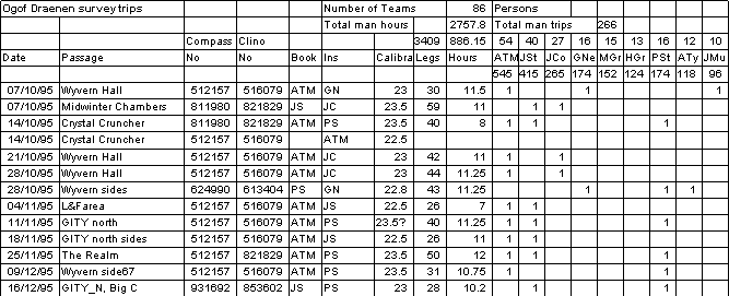 Table 1 - Surveys & Calibrations
On the fourth entry it seems as if ATM was on two trips but in reality it was one team. The second calibration with ATM on the instruments was required because a very low crawl was surveyed and the leap frog was maintained using two sets of instruments each with their own calibration (this needs careful book keeping, with an initial against each leg to state who was taking the reading.
The fifth from bottom has a ? next to the calibration. This day was foggy so no surface calibration was possible. The calibration figure used (23.5) was derived from PS calibrations with that set of instruments before and after that date (a comparison with a second set of instruments also helped set the figure)
Other sections of the table like duration of trip and who else took part, extend the table. We have found this gives a friendly competitive edge to getting more support by them knowing they are moving up the table and their effort is being noted. Other figures are just for fun e.g. Total time, No's of legs (cross check with survey), No's of trips by each person, Total no of teams etc. The prime importance is the calibration.
The second table was constructed to calculate the total length of the cave. This sounds like a complex task if one is to use the international length conventions. But in a table format the task is reduced to several simple steps.
Each page of notes from the grade 5 survey is represented by 1 row of the table. Each file (survex) of grade 2 data is also 1 row. Extra rows for data not received can also be included (grade 1).
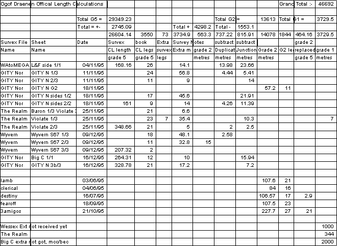 Table 2 - Cave Lengths
For each page of grade 5 notes the centreline(CL) length is calculated (frequently over several pages). The number of legs on the page is included as a cross check (the second column Extra survey legs, is for legs contained in the notes pages, not figures page of the notes and included in the CL length)
Additional columns have been added to this table to indicate which club did which part and also which sheet on the survey most of it appears on.
Passage is only counted if it is enterable, i.e. too tight rifts etc. don't count as passage. You have to remember that the length to side passages doesn't count either. As we continue with the grade 5 survey the proportion of extra length / centreline length decreases as it becomes more comprehensive. When I started constructing the table (around the entrance area), I found the length added was almost the same as that subtracted. It was not until I reached areas like Squirrel Rifts, The Realm or Wyvern Hall that a noticeable percentage increase was noted. I am sure this last table will make a few people think and hopefully cause some useful discussion.
by Robert Thrun
Copyright 1996 Robert Thrun
This article is being simultaneously published in both the UK 'Compass Points', and the US 'Compass & Tape'
A lot of cavers are starting to use Global
Positioning System (GPS) receivers to determine cave locations
with the intent of being able to easily find the caves again.
This article discusses the accuracy of GPS locations and two
methods to improve the accuracy: averaging and the use of two
receivers.
Background
The United States Department of Defense (DOD) has put up 24 satellites that make up the Global Positioning System. The GPS satellites transmit precisely timed signals along with their orbital co-ordinates. The GPS receiver measures the arrival time differences and uses them to get its location relative to the satellites' locations. The receiver gives its location in either latitude or Universal Transverse Mercator co-ordinates.
The advertising literature from some of the GPS manufacturers makes it difficult to get a simple answer to "How accurate is it?" Each manufacturer seems to state the accuracy in a different way: root-mean-square error, or circular error probability, and it is not clear if they are quoting nominal DOD specifications, giving best-case results, or giving worst-case results. The DOD accuracy specification could be quoted, but to get real-world accuracy figures, we have to actually log GPS results.
The accuracy of GPS is not as good as what most cavers would like. In particular, DOD imposes Selective Availability (SA) upon the signals sent down from the satellites. SA is a deliberate degradation of the accuracy of the signals so that they will be less useful to potential enemies. Very strangely, SA was turned off during the Gulf War and the Haiti invasion, two times when we would most want to confuse the enemy.
Many users want to get more accurate locations than are given by GPS with Selective Availability. The standard way of doing this is to use Differential GPS (DGPS). The US Coast Guard feels that better accuracy is needed for some harbour approaches, so they have set up a system of beacons to broadcast correction information. The DGPS receiver costs about $500 and connects to the GPS receiver. This is what is meant when a GPS receiver is advertised as "differential-ready". The Coast Guard beacons are located along the coasts and the Mississippi River, not in the mountain areas where we go caving. The Federal Aviation Administration plans to install DGPS beacons at airports. Thus we have the ridiculous situation where one government agency, the DOD, puts up a very accurate navigation system, deliberately degrades it, and two other agencies work to undo the degradation. There are some private companies that provide a broadcast correction service, but they do not yet cover the inland caving areas.
The Coast Guard DGPS supposedly provides accuracy to 5 or 10 meters. Even better accuracy can be had from GPS receivers meant for surveying use. Two-meter accuracy is claimed for the survey units. Somewhat better survey units can get accuracy of a few centimetres by using phase measurement techniques on the signals. Some really high-end units claim 0.5 mm accuracy.
The survey DGPS receivers store the raw data
from satellites, which can be post-processed to get the differential
corrections. Some of the units have sufficient internal memory
to store readings at 1-second intervals for most of a day. The
prices for the survey units start at about $3000. A phase-measurement
unit is over $5000, and prices go up to about $50,000. To do
DGPS, you need two receivers, but it is not necessary to buy two
receivers. Many states provide the service of fixed base stations
recording GPS data. Surveyors can subscribe to this data.
Bob Hoke bought a Garmin 75 receiver, and I bought a slightly newer Garmin 45. As of this writing, the Garmin 45 is one of the lowest priced receivers on the market at about $300.
Since the low end of the market is dominated by marine users, most of the receivers have a serial port that puts out a data stream in one or more of the formats specified by the National Marine Electronics Association (NMEA). The NMEA data stream may be captured by any communications program. The Garmin 45 gives latitude and longitude to 0.001 minute. The older Garmin 75 gives locations to 0.01 minute. The co-ordinates are given once approximately every two seconds. A program was written to convert the latitude-longitude data to meters in the Universal Transverse Mercator (UTM) system and subtract the average for the session. In all the figures in this article, the average location has been subtracted from the data.
Many GPS receivers can periodically store locations as waypoints along a track. The stored waypoints can be downloaded to a computer using a proprietary protocol. This does not require carrying a computer into the field. For this study computers were used to capture the NMEA data stream in order to collect the maximum amount of data.
Figure 1 shows the data that were obtained from the Garmin 45 during a 50-minute session on February 12, 1995. The three plots on the left show the individual north, east, and altitude components of the location after the average location was subtracted. The plot on the right shows the map view (north and east) co-ordinates. The receiver was stationary during the session, but it gave a location that wandered around. The GPS locations could be enclosed in a 70 by 100 meter rectangle. The average was about 11 meters from the location that was read as carefully as possible from a 1:24000 topographic map.
The variation is rapid enough so that we can't go from a benchmark, to the cave, back to the benchmark and then interpolate with time to get the correction. This is what we would do with altimeters, because atmospheric pressure varies slowly, but GPS locations vary too rapidly.
The less technical descriptions of DGPS make sound like it is simply a matter of taking the difference between the co-ordinates from two receivers. Most cavers can only afford the cheap GPS units. We thought that it should be possible to do DGPS by logging the co-ordinates from two cheap units to computers. When I called one of the manufacturers about this possibility, the technician pointed out that the two receivers must be using the same set of satellites. The cheap receivers will accept the differential corrections, but they will not put out the corrections. Some of the more technical literature points out that the order of correction operations is important and that the corrections should be applied to the raw data. The survey systems do post-processing with the raw survey data. Obviously, the cheap GPS units must be using the raw satellite data internally, but they do not put that out. I suspect that there are only a few lines of firmware and a fair chunk of memory difference between the marine units and the survey units. Some manufacturers even use the same plastic cases.
Despite the suggestions that it might not be the best way to do things, we decided to try a Do-It-Yourself (DIY) DGPS with two cheap receivers on the possibility that might provide a significant improvement over the accuracy of a single receiver. On May 6, the Garmin 45 was set up in the same location as in February. This was a near-ideal site. It was on the roof of a car in a large empty parking lot. Seven or eight satellites were usable at all times. Data were logged for over 2.5 hours. The co-ordinates with the average subtracted are shown in Figure 2. The spikes at around 900 seconds are due to experimenting with battery-saver mode while the unit was running. Again, the co-ordinates could be enclosed in about a 70 by 100 meter rectangle. The averaged location was 15 meters from the location that was read from the topo map and 5.95 meters from the February average.
Also on May 6, the Garmin 75 was set up near a house in a residential neighbourhood about 11 kilometres from the Garmin 45. The Garmin 75 location had houses and trees as obstructions. Its data were logged for a longer period that overlapped the Garmin 45 data, so we are able to make a comparison at the same times. The co-ordinates with the average subtracted are shown in Figure 3. Because the latitude and longitude were reported to 0.01 minute at the serial port, the co-ordinates change in steps ten times larger that the Garmin 45. A 0.01 minute rectangle is 14.411 by 18.498 meters. The Garmin 75 reports to better accuracy on its front panel display. The co-ordinates from the Garmin 75 varied more than the Garmin 45. The section starting at about 4500 seconds where the altitude does not change indicates that the unit could not see the four satellites that necessary for 3-dimensional navigation and went into 2-D mode. Because of this data and because we could see obstructions, we are sure that the two units were not seeing the same set of satellites.
When we compare Figures 2 and 3, we can see that there is a high degree of correlation between the co-ordinate variations of the two receivers at some times, but there are also times when they differed greatly. The differences between the Garmin 45 and 75, again with the average subtracted, are shown in Figure 4. The differences do not show much of an improvement over the raw data. Even where it looks like the two units are dead on, as for the altitudes around 2500 or 3600 seconds, there is about a 20-second difference between the curves. The lag might be related to the fact that the Garmin receivers do multiplexing. The conclusion is that this attempt at DIY DGPS did not work. Another trial with identical receivers where both have good coverage might work, but we certainly can't count on it. We can only hope for the prices on surveying GPS units to come down. The only real difference between marine units and survey units is the internal memory for saving raw data.
A comparison with the average tells us about
consistency, not accuracy. Reading a location from a map has
errors of its own. To get an idea of absolute accuracy, the Garmin
45 was set up at a geodetic benchmark on Spruce Knob, the highest
point in West Virginia, on September 4, 1995. Receiving conditions
were good, with 6 or 7 satellites in use at all times. The results
of that session are shown in Figure5. The latitude and longitude
of the benchmark were got from the National Geodetic Survey.
The averaged GPS location was 11 meters due west of the actual
location. The logging was interrupted to save the data to disk,
giving four sessions of 15, 16, 18, and 31 minutes with locations
23, 9, 20, and 3 meters from the actual location.
It is evident that the average locations are reasonably accurate. How often and for how long should we sample? I'll express my opinion. You should refer to the figures to follow my reasoning.
The sampling should be frequent enough so that more frequent sampling will not change the average. This means that we should have points on all of the peaks and during times of rapid change. The maximum number of waypoints that can be stored in the GPS receiver could limit the number of samples that can be taken. Otherwise, we would just sample as frequently as possible. From the figures, it looks like every 10 to 30 seconds is a reasonable rate.
The duration must be longer than the longest
peak. Otherwise, we might as well just take one reading. A 10
minute session would get the average off the peak. The duration
should cover at least one complete cycle of the longest-period
co-ordinate changes that we see in our logs in order to get a
zero average for a cycle. More cycles would be better. The co-ordinate
changes are very irregular, but it looks like a 30-minute logging
session would cover the longest cycle.
A single GPS location has 50 to 100 meter accuracy. Averaging can increase the accuracy to 10 to 20 meters. The data should be averaged for at least 30 minutes with 10 to 30 seconds between samples, with 10 minutes being the shortest period for which averaging is of any benefit.
The traditional way of locating caves is to plot their location on topographic maps and measure their co-ordinates on the map. If good maps are available and locations can be plotted relative to easily distinguished topographic features, the traditional method is better than GPS. There are some valid reasons for using GPS, such as featureless areas or areas with poor maps. Until Selective Availability is turned off or the price of surveying GPS units comes down, we will continue to use topographic maps as the primary method for locating caves with GPS as a check for blunders.
_________________________
PS The White House announced on March 29, 1996 that
the most precise GPS data will be made available to civilian users.
Press accounts did not make it clear exactly what this would
involve. The military has two channels of encrypted Precision
Code (P-code) on two different frequencies. Civilians have another
channel of Coarse Acquisition (C/A) signals. The C/A signals
are inherently less accurate than P-code, and the C/A signals
are further degraded by Selective Availability. The new policy
will be phased in over four to ten years. Selective Availability
could be turned off in a few hours as the GPS satellites pass
over ground stations. Use of the P-Code would require a new generation
of receivers for civilian use.
Figure 1. Data collected with Garmin 45 on February 12.
Figure 2. Data collected with Garmin 45 on May 6.
Figure 3. Data collected with Garmin 75 on May 6
Figure 4. Difference between Garmin 45 and 75 data at two locations, 11 km. apart.
Figure 5. (Front Cover) Data collected with Garmin 45 on Spruce
Knob, September 4.