
five-hour GPS plot showing how the readings wander, and that the geometric mean is likely to be a better position estimate than any of the individual readings.
Compass Points is published quarterly in March, June, September and December. The Surveying Group is a Special Interest Group of the British Cave Research Association. By subscribing to Compass Points you will automatically become a member of the CSG and will receive its quarterly journal. The CSG's publishing agent is the Cave Radio & Electronics Group (CREG). CREG also publishes a quarterly technical journal to which you can subscribe if you want to. Subscriptions to Compass Points should be made payable to CSG, and sent to the secretary, Andrew Atkinson. Further details below. IF you also wish to subscribe to CREG the two can be done together, with the cheque made out to CREG and sent to their secretary David Gibson. Information sheets about the CSG and CREG are available. Please send an SAE or Post Office International Reply Coupon.
NOTES FOR CONTRIBUTORS
Articles can be on paper, but the preferred format is ASCII text files with paragraph breaks. If articles are particularly technical (i.e. contain lots of sums) then Microsoft Word documents (up to version 7.0) are probably best. We should be able to cope with most common PC word processor formats. We are able to accept disks from other machines, but please check first. We can accept most common graphics formats, but vector graphic formats are much preferred to bit-mapped formats. Photographs should be prints, at actual size, and non-returnable (so we can cut them). Alternatively, well scanned photos (e.g. from a PhotoCD) supplied as .BMP or .PCX files are OK. It is the responsibility of contributing authors to clear copyright and acknowledgement matters for any material previously published elsewhere.
COMPASS POINTS EDITOR Wookey
734 Newmarket Road, CAMBRIDGE, CB5 8RS. Tel: 01223 504881
E-mail: wookey@aleph1.co.uk
SUBSCRIPTION & ENQUIRIES Andy Atkinson
c/o 38 Delvin Rd, Westbury-on-Trym, BRISTOL, BS10 5EJ
Email:a@atkn.demon.co.uk
PUBLISHED BY
The CAVE SURVEYING GROUP of the BCRA.
OBJECTIVES OF THE GROUP
The group aims, by means of a regular Journal, other publications and meetings, to disseminate information about, and develop new techniques for, cave surveying.
BCRA ADMINISTRATOR
20 Woodland Avenue, Weston Zoyland, BRIDGWATER,
Somerset, TA7 0LQ
COPYRIGHT
Copyright (c) BCRA 1996. The BCRA owns the copyright in the layout of this publication. Copyright in the text, photographs and drawings resides with the authors unless otherwise stated. No material may be copied without the permission of the copyright owners. Opinions expressed in this magazine are those of the authors, and are not necessarily endorsed by the editor, nor by the BCRA.
ANNUAL SUBSCRIPTION RATES (amendments May 1996)
Publication U.K. Europe (air) & World:
World:surface Airmail
CSG Compass Points 4.00 5.50 8.00
CREG Newssheet only 2.50 2.50 3.50
CREG Journal 8.50 10.00 12.50
Journal and Compass Points 10.00 12.00 15.00
These rates apply regardless of whether you are a member of the BCRA. Actual "membership" of the Group is only available to BCRA members, to whom it is free. You can join the BCRA for as little as £3.00 - details from BCRA administrator. Send subscriptions to the CREG secretary. Cheques should be drawn on a UK bank and payable to BCRA Cave Radio & Electronics Group. Eurocheques and International Girobank payments are acceptable. At your own risk you may send UK banknotes or US$ (add 20% to current exchange rate and check you don't have obsolete UK banknotes). Failing this your bank can "wire" direct to our bank or you can pay by credit card. In both these cases we have to pay a commission and would appreciate it if you could add extra to cover this.
DATA PROTECTION ACT (1984)
Exemption from registration under the Act is claimed under the provision for mailing lists (exemption 6). This requires that consent is obtained for storage of the data, and for each disclosure. Subscribers' names and addresses will be stored on computer and disclosed in an address list, available to subscribers. You must inform us if you do not consent to this.
COMPASS POINTS LOGO
courtesy of Doug Dotson, Speleotechnologies.
INTERNET PUBLICATION
Published issues are accessible on the Web at http://www.chaos.org.uk/survex/CPIDX.HTM
THE CSG Web pages are at http://sat.dundee.ac.uk/~arb/CSG.html
Larry Fish
Discussion on the limitations of Least Squares in dealing with blunders and discussion of what should be done instead.
Wookey
Details of practical GPS use in the field, and how to process the data afterwards.
This will be the CSG's inaugural field meet as a separate group. Note that this was advertised as being in March in the last issue of the journal. That has been moved to 12th-13th June to avoid a clash with the BCRA Science Symposium, on the 15th March. See the display ad on p11 for further details.
Planning for the meet is well in hand with permits for Leck fell and Casterton fell booked. We need people to actually stick their hands in the air to say they are coming and if anyone would like to do something useful to help then please contact Pete Grant. Useful things to do include: Leading the 'beginners cave surveying' trip down Bull Pot of the Witches (within easy cup-of-tea distance of the Red Rose Farmhouse), Surveying down as much as possible of Lost Johns and Notts Pot. Rigging in or out of Lost John's/Notts to facilitate surveying, Providing some proper theodolite gear/expertise for surface surveying the Casterton Fell entrances. If anyone has their own projects/experiments they would like to do then please tell Pete or Wookey if there is anything you need in advance.
PCs, RISC PC and OHP will be available.
Our Secretary, Andy Atkinson has a new email address that actually works now, so enquires to that should produce a response.
Pete Grant is now field meet organiser and publicity officer.
Richard Rushton (of CREG), is now the Special Interest Group representative on BCRA council.
If you, or your Club want to join the cave surveying group, then please send remittance to the new keeper of the list, Andy Atkinson - address given in the Masthead.
We have 97 members at last count, about ¾ being also members of CREG.
The CSG will be at the UIS conference, and the surveying meetings afterwards. We'll report back what goes on. There will be a 'Map Salon' at this event where your maps will be judged against the rest of the World by an international panel. The categories are:
Yvo Wiedman asks for as many entries as possible. So, if you or your club have ever drawn up a decent survey, then please consider entering. It doesn't cost anything, but we do need to reserve space. I will be able to transport it to the conference and display it. There are certainly some very good surveys about….
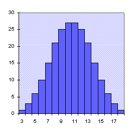
Compass Point 14 had an error in the graph to illustrate what happens when you throw 3 dice, 'cos I got the sums wrong. It should have looked like this:
Survex has had some new releases, which is good because the old versions have all timed out and will now put up irritating 'this software is out of date' messages. The next release of Survex will have this reminder removed as it is now sufficiently mature that it isn't necessary.
The new release is v0.71 which is really v0.70 tidied up and released properly. The UNIX /Source and DOS(386) variants are already online. The DOS(286) version will follow, and the RISCOS (v0.72) release should be uploaded by the time you read this.
A new example dataset is also available which better illustrates many of Survex's more powerful features, and ways of doing things. This is based on CUCC's Austria dataset with some of the sensitive stuff taken out.
Also now available is the DOS(386) version of caverot which has been in gestation since v0.60. This finally removes the DOS 640K limit on caverot datasets on PCs, and allows SVGA (800x600x256) to be used. It is still very new and we would like feedback about how well it does or doesn't work on your system.
The web pages containing all of this software can be found at:
http://www.chaos.org.uk/survex/SVXHome.htm
You can also get copies by sending a formatted floppy to Wookey at the editorial address. Registered Users will be updated automatically.
A number of people round the world are working on this, and various pretty pictures are starting to appear. Mike McCombe (of Speleogen fame) is working on putting out VRML as well as DXF, and already has software producing VRML output. Julian Todd has written Tunnel. This is intended to provide the full 3d visualisation features lacking in Survex. It is written in Java for portability, and has some advanced concepts. I was hoping to show you what it can do in this issue of CP, but it looks like it will have to wait till next time…
Garry Petrie and Alan B Canon have also both produced VRML cave pictures, and this is clearly going to be a popular idea.
This software has had four releases in the last 12 months, with some major improvements. Here is what Larry has to say about the latest version.
Larry Fish
FINALLY, the process of porting COMPASS from DOS
to Windows is complete and all the pieces are in place! To celebrate,
I have a special free registration offer that lasts through February
28, 1997. See item six below for details.
Here are the new features:
1. NEW LOOP CLOSER. The Windows version of COMPASS
now has the ability to close survey loops. The program will close
survey files of almost unlimited size. File size is only limited
by the amount of free memory on your computer. Generally speaking,
the closer will process about 100 miles of cave per megabyte of
free memory. The Loop Closer is also extremely fast. It will close
all the loops in Lechuguilla in two minutes on 90 Mhz Pentium
computer.
The COMPASS loop closer was specially designed to
deal with blunders and gross errors. Blunders are one of the biggest
problems in cave surveying. Even when a cave is very carefully
surveyed, 30 to 50 percent of the loops have blunders in them.
For example, 32% of the loops in Lechuguilla Cave have errors
greater than two standard deviations. This means that at least
one shot in 50 has a gross error or blunder in it. As another
example, a study of a the recent resurvey of Cave of the Winds
shows that even when you are very careful, one in 20 shots has
a blunder.
As a result, loop closing software must be able to deal with blunders. Most programs use a process called Least Squares/Simultaneous Equations. This process distributes survey errors across all the loops in the cave. Unfortunately, this means
that gross errors and blunders from the bad loops
contaminate the good loops. COMPASS uses a special technique that
closes the best loops first and then locks them down so that they
cannot be contaminated by the bad loops.
2. NEW WINDOWS PROJECT MANAGER. COMPASS now has a
new Project Manager that automates all aspects of the surveying
process. The Project Manager performs two main functions. First,
it allows you to organise and structure cave surveys. Second,
it completely automates the processing of cave data.
COMPASS gives you great flexibility in organising your cave survey data. Data can be organised as multiple hierarchical trees of data. The Project Manager organises cave data by displaying a "tree" diagram of all the surveys, files, and caves in your project.
Creating, organising, selecting and processing is
a simple point-and-click process.
COMPASS also has special features that allow you
to combine large caves or cave systems into a single image. "Local"
and "global" linking features mean that you can combine
caves even if there are duplicate station names in different files.
Also, individual survey files can participate in more than one
project. This means that you have complete flexibility in how
you organise and display data.
3. THE DEM READER. The DEM Reader will now handle
7.5 minute digital elevation model maps. The data in the 7.5 minute
maps is much higher resolution than the one degree maps. The data
in the 7.5 minute maps is spaced only 90 feet apart instead of
300 feet apart in the one degree maps. This means that these maps
will more accurately reflect small variations in the surface terrain
above your caves.
4. DOCUMENTATION. There are now more than 200 pages
of documentation for the Windows version alone. In addition, the
DOS version has more than 200 page of documentation.
5. THE EDITOR. As a part of the "survey repair"
features, the Editor now has the option of fixing shot information
that has been entered in the wrong column. For example, if the
Editor was set for Up, Down, Left, Right survey order, but the
book was actually, Right, Left, Down, Up order, the data would
be entered in the wrong column. Normally, you would have to re-enter
the data, but with this option you can swap columns for any two
numerical items. This can be done for part or all of a survey.
6. SPECIAL FREE OFFER. With the completion of the
Windows version of COMPASS, there is now a separate registration
fee for the Windows version. Registration for the DOS version
is still $25 and the Windows version is an additional $25. If
you register both at the same time, the combined registration
fee is just $38. To encourage everyone to register, anyone who
has registered the DOS version before February 28, 1997 automatically
gets the Windows registration FREE OF CHARGE. If you have already
registered the DOS version anytime in the past, you are automatically
upgraded free of charge.
HOW TO GET COMPASS
COMPASS is a shareware product. You can try it out free. If you like it and want to use it, you must register. If you don't like it, then don't use it and pay nothing.
The registration cost is $25.00 for the DOS version and $25 for the Windows version. Combined registration is $38. Anyone who has registered the DOS version before February 28, 1997 is automatically registered for the Windows version.
COMPASS is available free of charge for evaluation purposes. Copies are available through the COMPASS World Wide Web page at:
http://www.usa.net/~lfish/compass.html
The Web Page also has full colour screen images of
some of the most important features. It also has connections to
other cave related WWW pages including links to the USGS DEM files.
The whole COMPASS package has hundreds of features and a full
description of the software is beyond the scope of this document.
However, the COMPASS Web Page also has a complete and detailed
description of all the features and options.
[Ed: Not wishing to detract from Compass which is excellent software doing many things Survex doesn't do, but it is worth noting that Survex has always (ref. numbers above) 1 (had loop closure only constrained by machine memory), 2 (had 'Project' files to organise and automate data processing), 5 (had Specifiable data ordering, so you don't need a feature to swap data around in the editor), 6 (been Free).]
Garry Petrie
The capabilities of today's cave surveying software is truly amazing. There are several quality offerings for the cave surveyor.
Rather than list all of the features these programs
have in common with WinKarst, here are some important differences.
WinKarst comes in 16 and 32 bit versions for Windows 3.1 and '95.
It comes as a self extracting setup program. It can reference
caves by geographic longitude/latitude co-ordinates and automatically
find the correct magnetic declination for that location. WinKarst
can export GPS data for uploading and three dimensional DXF cave
descriptions. It can operate on different objects, caves, loops,
surveys within a cave survey. WinKarst can accept drag-n-drop
files from the File Manger or Explorer and can be started by double
clicking on a cave survey file icon.
Here are the important changes for current version:
Improvements
- Garmin track and waypoint export
Two new types of file exports are now supported, Garmin track (TRK) and waypoint (WPT). The exported file can be uploaded
with Garmin's PCX5 software. A cave's control points
and extents are exported as waypoints, while a simple line plot
is created as a track. For this option to work, a geographic location
must be specified in the raw survey file. The exported text file
format is only compatible with Gamin's software, but simple editing
can translate the file to other track and waypoint formats.
- Colour properties in DXF export
Colouring options such as colouring by survey or
colour by time are now encoded into the DXF file exports. This
makes the visualisation of complex passages easier. Note, the
exact colour shown in a program importing a WinKarst exported
DXF file are dependant upon the importing program's colour map
and not on WinKarst's.
- Usage of ellipsoids and datums
The previous version of WinKarst actually only specified
various Earth ellipsoids for its map projections. WinKarst now
includes 23 different Geodetic Datums, which in their definitions
specify a particular ellipsoid. This should reduce confusion in
specifying map co-ordinates and including GPS readings since these
sources usually reference a datum rather than an ellipsoid.
- Datum statement in raw data file
Geodetic co-ordinates, longitude and latitude, should
also include a Datum from which they're referenced from. This
facilitates data exchanging and accurate plotting on topographical
maps. A #DATUM <name> statement has been added to the raw
survey specification. The name values are consistent with names
recognised by Garmin's GPS units.
More info at:
http://www.europa.com/~gp/winkarst.html
All the above software is available from the editor if you don't have net access: Send 1 (1.4Mb) floppy for each of: Survex or Compass for DOS or Compass for Windows. Send three floppies for WinKarst. I've also got a ZIP drive now, so if you want to have a pile of everything then send me a ZIP disc.
P.R.Cousins
There are two points in John Stevens' article 'The Chelsea Surveying Ethos' in Compass Points No. 12 that cause me some concern.
[apologies to Pete for my missing this out last issue - Ed.]
Andy Waddington
I have been looking at the proposed standard symbols for cave surveys, something which on the face of it, seems like an excellent idea. I was expecting someone would start a discussion on the topic, but as no-one else has, here are a few comments to throw about...
Many of these symbols are familiar, and I wouldn't argue with most of these or several of the less familiar ones. However, some groups of symbols give me some considerable concern.
Well, I have never seen any of these symbols before. They are not at all like the old CRG (and later BCRA) ones. I very strongly dislike them because they depend on the orientation of the survey drawing (I am talking about the plan, not the elevation). Now, for a surface topographical map, it is conventional to map a rectangular (-ish) area, and to have north to the top.
This is a standard orientation, which everyone understands. Equally, the mapped area of a cave often does not conveniently fit into a rectangular area with one edge aligned north-south. Very commonly, as new parts of the cave are explored and the survey updated, the cave drawing has to be rotated to be a sensible fit onto rectangular paper. Often this rotation can be quite large, and symbols such as these will no longer look the same - they may even end up being confused with each other. The old CRG/BCRA symbols could be rotated as far as you liked without needing to redraw, but still remained essentially the same. Admittedly, they weren't very obvious, but they do point up the need for a non-orientation-dependent symbol.
This symbol also is nothing like the older British standard one, but the fact that you can omit the arrow if unsure of the direction is a good one, so I do approve of this replacing the older UK one.
This is an old and very familiar symbol. Don't forget, though, that it is not what cave divers use. Obviously, as most of their surveys are underwater, they don't want the entire passage detail hidden by cross-hatching! Here, it is understood that the passage is a sump, without a special symbol. Some sort of note to this effect would usefully accompany this symbol in the standard.
This is unlike the majority of surveys drawn in the UK. I personally find surveys drawn this way extremely hard to read, and the lines confuse all the other passage detail. I know other people find them useful, so wouldn't want to outlaw them, but could they not be one of two alternative ways of representing gradients? The tapered triangular slope-marker of British surveys is much more useful when superimposed over boulder slopes (where contours would be almost impossible to draw anyway). They also work fine for small slopes which might be smaller than your chosen contour vertical interval.
I note that no symbol is presented for 'bare rock' which the Americans have. How are we to distinguish between 'bare rock' and 'floor detail not recorded' ?
Often, a route is marked in the cave by flagging tape, or perhaps only by previous footprints. Should we have a symbol to show this ? or to mark that a certain passage has been looked at, doesn't go, and is fragile and should not be crossed again?
The old British symbols used to have separate symbols for the entrance dripline, and for the limit of daylight. What happened to these?
Similarly, the old British symbol set had a specific symbol for when a passage had no wall - it just got lower and lower in a bedding until cavers could get no further - the symbol represented the furthest limit that could be seen to still be passage.
Things like extent of ice and snow, the directions of draughts and one or two other things, are flagged with a date. This is very sensible, but there are standards already for dates. Americans use a different one from Europeans, and far too few people use the International one! If we are proposing an international symbol set, can we please agree to use an international date format? The ISO standard "Format of dates for information interchange" very sensibly specifies the format yyyy.mm.dd (with times hh:mm:ss etc. to follow).
As Wookey notes in Compass Points, using letters to convey meaning is very language-dependent. 'P' means 'Pitch', 'Pit', 'Puits' etc. and is close to international (unless you say 'shaft' or 'schacht' , but the other letters are much less meaningful. 'C' to an English reader means 'Climb', with the symbols on the survey making it clear which way is up. 'R' is quite unfamiliar to English-speakers, though many of us in Europe have got used to it meaning 'Climb'. I had never heard of a distinction between a climb discovered from the top and bottom before. Surely an aven (dome in the US) is just a pitch (pit in the US) found from the bottom... if it goes, then its symbol is going to depend on which way one comes upon it?
I feel that these various possibilities must be distinguished graphically (and without reliance on the orientation of the plan . Existing symbols should be enough to show the difference between an up and a down. Maybe some sort of symbol alongside would distinguish drops which need gear?
That still leaves a problem with a wide vertical where there is a climb at one point, or a roped or laddered route at another...
There is a risk of trying to show too much on the survey, which risks de-emphasising the accompanying descriptive article, though clearly, the latter is also a problem if your audience speaks many different languages...
Good caving,
Andy
In the Cavers Digest Email list Paul Smyth said:
There would be advantages to an international standard for cave cartography but such a standard should not just include symbology. It should also specify the size, orientation, stroke widths and colour for the symbol. YES Colour! We should adopt a standard which also specifies the colours to be used on surveys. Printing in colour used to be prohibitively expensive for an activity such as caving but this is no longer the case.
Discussion in following issues concerned mainly the feasibility or advisability of colour cave maps versus black & white, rather than actual colour standards.
Ken Grimes, writes:
Firstly I agree that coloured maps are difficult to reproduce cheaply and should NOT be used for normal purposes. At least, not until colour photo-copiers occur at every newsagent's shop.
However, it is worth considering how we would use colour and how it would help (if at all). And it is best to think about standards now, than too late when everyone has created their own independent set.
Some suggestions:
(1) Avoid excessive colour.
It just makes for a garish map and remember some of us are colour blind. Most of the map symbols should be kept black & white with colour only used where it helps to reduce confusion in complex situations.
(2) Use specific colours for related GROUPS of symbols or themes.
(A) Differentiating passage levels in a cave with multiple overlapping levels (mainly in small scale maps) by using a colour fill within the walls of the passages, or by colouring the wall lines themselves (larger scale maps). There are two approaches to this. (i) Use a rainbow scheme with red for the highest level through to violet at the lowest level (or visa-versa) or (ii) use pale colours for higher levels and darker (or brighter) colours for the progressively lower levels. This latter scheme allows the (darker-coloured) lower levels to be seen below a (pale-coloured) broad high-level chamber.
(B) Differentiating groups of detail symbols where these are superimposed (mainly in large scale maps). This solves the problem where the surveyor wants to show both roof and floor detail, not to mention sediment types etc. Things can get quite unreadable in black & white.
Symbol Groups that could be given distinctive colours are:
(i) Roof detail (roof steps, roof channels, stals(?) etc.)
(ii) Floor topography (steps, pits, slope arrows, ....)
(iii)Floor composition (hatches/stipples for mud, sand, gravel, rubble; and possibly also guano etc.). I prefer to leave bedrock blank, as all the symbols I have seen suggested for it have been too overbearing and clashed with the other floor details etc. The colour used here should be one that is paler than the others so that the patterns do not obscure the other detail - perhaps a mid to light brown?
(iv) Water features. Probably in blue as that is traditional on topo maps.
(v) Surface features (contours, property boundaries, ...). Use a pale colour.
That is five line colours already, plus black - probably the limit for easy readability?
(vi) Decorations (stals etc.) might best be left black?
(vii) A colour should perhaps be reserved for special purpose maps which are showing something unusual that needs to be in a distinctive colour.
(viii) All symbols that do not fall in the above groups should be left as black.
Note: at this stage I am not suggesting specific colours, let's sort out the essential colour groups first - and let's not have too many groups or we will run out of useable line colours. Note that, when used in thin lines, some colours (hues) are difficult to distinguish unless they are particularly bright (high chroma); e.g. blue and green. Red-orange-brown can also be difficult unless they are also at different intensity (value).
(3) The symbols themselves should not change from those already in use on colour maps (or from those we settle on in the UIS proposal).
(4) Warning text could be in red? "Here be Dragons"
(5) A pale background wash could be useful in the non-cave (solid rock) areas of the map. This will make it easy to follow what is pillar and what is passage in those confusing phreatic spongeworky areas.
(6) Anyone creating a colour map should make a test
photo-copy to ensure that it is still readable in black &
white. This assumes that you are drafting in CADD, and it is
easy to change the colours if you find they don't work!!
Larry Fish
Most cave surveyors assume that the best way to close a loop in a cave is to use an algorithm based on the "Least Squares/Simultaneous Equations" (LSSE) method. This is probably due to the fact that LSSE itself is based on sound mathematical and statistical methods and is widely used by land surveyors. It also partly due to the fact that it has the aura of being a complicated, sophisticated and esoteric algorithm. This idea is so pervasive, that no one ever examines the possibility that LSSE might have flaws when it comes to cave surveying. This is exactly why I am writing this article. I think that LSSE, although mathematically sound, is not the best method of CLOSING cave survey loops. I think that it is a very good tool being used for the wrong job.
Here is my argument in a nutshell: LSSE is a very powerful mathematical and statistical method with many uses. But, in terms of CLOSING cave loops, Least Squares/Simultaneous Equations is best suited for dealing with random errors that are evenly distributed across the whole cave. However, evenly distributed, random errors are not the biggest problem in cave surveying. Localised blunders are the biggest problem in cave surveying and LSSE does not handle blundered loops very well.
Let me give you some background. There are three kinds of errors that occur in cave surveys: random errors, systematic errors and blunders.
Random errors are small errors that occur during the process of surveying. They result from the fact that it is impossible to get absolutely perfect measurements each time you read a compass, inclinometer or tape measure. For example, your hand may shake as you read the compass, the air temperature may affect the length of the tape, and you may not aim the inclinometer precisely at the target.
There are literally hundreds of small variations that can affect your measurements. In addition, the instruments themselves have limitations as to how accurately they can be read. For example, most compasses don't have markings smaller than .5 degrees. This means that the actual angle may be 123.3 degrees, but it gets written down as 123.5.
All these effects add up to small random variations in the measurement of survey shots. Around a loop, these random errors accumulate and cause a loop closure error. Even though these errors are random, the accumulated error tends to follow a pattern. The pattern is called a "normal" distribution and it has the familiar "bell" shaped curve. As a result of this pattern, we can predict how much error there should be in a survey loop if the errors are the result of small random differences in the measurements. If a survey exceeds the predicted level of error, then the survey must have another, more profound kind of error.
Systematic errors occur when something causes a constant and consistent error throughout the survey. Some examples of systematic errors are: the tape has stretched and is 2 cm too long, the compass has a five degree clockwise bias, or the surveyor read percent grade instead of degrees from the inclinometer. The key to systematic errors is that they are constant and consistent. If you understand what has caused the systematic error, you can remove it from each shot with simple math. For example, if the compass has a five degree clockwise bias, you simply subtract five degrees from each azimuth.
Systematic errors are usually dealt with by calibrating instruments on a survey course, or by adding correction factors to the survey data.
Blunders are fundamental errors in the surveying process. Blunders are usually caused by human errors. Blunders are mistakes in the processing of taking, reading, transcribing or recording survey data.
Some typical blunders are: reading the wrong end of the compass needle, transposing digits written in the survey book, or tying a survey into the wrong station.
Blunders are the most difficult errors to deal with because they are inconsistent. For example, if you read the wrong end of the compass needle, the reading will be off by 180 degrees. If you transpose the ones and tens digits on tape measure, the reading could be off by anything from 0 to 90 feet.
Blunders are extremely common in cave surveys. For example, in Lechuguilla Cave, 32 percent of the loops have blunders in them. In Wind Cave, 25 percent of the loops have blunders in them. (These are a conservative figure, because it is impossible to tell whether each loop has only one blunder in it.) By extrapolating I have concluded that in surveys like these, there is at least one blunder in every 40 shots.
Paul Burger did careful study of blunders during of a recent resurvey of the commercial section of Cave of the Winds. He found that one in 20 shots had a blunder. These figures are impressive, because these surveys were very carefully done in relatively easy, well lit, concrete-trailed walking passages. In more difficult caves, the blunder rate goes up rapidly. For example, in Groaning Cave, a cold, wet, alpine cave whose entrance is at 10,000 feet (3050 meters), 50 percent of the loops are blundered. All of this means that any survey with more than a few hundred shots, must have several blunders in it.
Let's start by looking at some of the characteristics of random errors. First of all, random errors, by their very nature, tend to be small. For example, you wouldn't expect to find random errors more much greater than an inch, a tenth of a meter or a degree in each shot.
The second important characteristic of random errors is that, over the long run, they have a tendency cancel each other out. This is easy to see. For example, if your errors are truly random, sometimes you may read the compass slightly positive. Other times you may read the compass slightly negative. The net effect is the positives and negatives cancel out. Taken together, these two characteristics mean that the total error in loops with only random errors is relatively small.
The LSSE method is designed specifically to deal with random errors.
It is in fact the best method of dealing with random errors. But if you have a survey that has ONLY random errors, it makes very little difference which algorithm you use! This is because the errors are so small that even a relatively simple algorithm will work as well as LSSE. In other words, there is no particular advantage to using LSSE if you have random errors.
Let me give you a real world example. I extracted a 1000 foot loop from Groaning Cave that had a relatively random looking error pattern. It was 64 stations long and had a 9 foot closure error.
Analysing the loop gives a standard deviation of about 1.0 (given a two degree variability in azimuth and inclination and .1 foot variability in length.) If you are not familiar with the concept, a standard deviation of 1.0 means that the error is about what you would expect if the errors are random. I closed this loop using both COMPASS and SMAPS and compared the result. SMAPS uses LSSE and COMPASS does not, so it a good way to analyse the difference. The maximum difference between the two loops was less than .1 of a foot.
I also did another experiment using a 2000 foot connected network of three loops of similar quality. The differences between SMAPS and COMPASS were less than .3 feet.
Now lets look at blunders. One of the big selling points of LSSE is that it closes all the loops in the cave at simultaneously. This is exactly what you want when you have evenly distributed random errors, but with blunders it causes problems.
Let's look at this in detail. LSSE handles blunders in exactly the same way it handles errors. That is, it distributes them evenly across the cave. This would be fine if all the loops in the cave were either all good (with only random errors) or all bad (with only blunders), but that is rarely the case.
In the real world, most cave surveys have a mixture of both good and bad loops. If you have some good loops and some bad loops, least squares will take the errors and distribute them more or less evenly across both the good and bad loops. This has the effect of contaminating the good loops with errors from the bad loops.
One way to deal with this problem is to design the LSSE algorithm so that you have independent control over how the program adjusts each shot. This is usually called something like the "confidence factor" and most LSSE implementations have this feature. Basically, you adjust this "confidence factor" to compensate for good and bad shots, surveys and loops. In other words, you give a higher confidence factor to the shots in the good loops and a lower confidence factor to the shots in the bad loops.
This almost works, except that you have a new problem: there will always be some shots that are shared by both good and bad loops! This creates a logical contradiction: you can't have a shot that is both good and bad at the same time. You could deal with this by setting the confidence factor for shared shots to a value halfway between a good and bad confidence factor. But, once again this would degrade the good loops by allowing a bad loop to alter shots in the good loop. The process is even more complicated if you have lots of loops which share common shots.
The way you close loops has a profound effect on the accuracy of cave statistics. This is true anytime you have two parallel loops connecting parts of a cave. For example, let's say that you are trying to determine the depth of a cave and there are two loops that connect to the deep point. One loop closes very well, and the other loop has an large blunder in it. Obviously, to get the most accurate measurement of the cave's depth, you want to ignore all the shots in the blundered loop and only use the shots in the good loop. If you use LSSE, the errors from the blundered loop will contaminate the good loop degrading the accuracy of the depth measurement.
Some people say, that you shouldn't even try to close blundered surveys, and there is a good argument to be made for simply discarding all blundered loops and immediately redoing the survey.
In fact, some survey programs refuse to close any loop that has a large error and appears to be blundered.
I think that blundered loops are exactly the reason you need loop closure. If a loop is good, it doesn't need much help from a loop closing algorithm. But if the loop is bad, it needs lots of help just to make the data even minimally useful.
The problem with discarding blundered surveys, is that it is difficult to get people to go back and resurvey caves. I have been trying for more than 10 years to get people to go back and resurvey the front part of Groaning Cave. Look at Lechuguilla. There are 245 loops with errors greater than three standard deviations. Wind cave has 132 loops with errors greater than three standard deviations.
Chances are very slim that you are going to get people back in these caves to fix all the loops. For one thing, cavers aren't very excited about re-surveying old passages. For another, the old survey stations are often lost, unreadable or moved, making the resurvey process much more complicated than just re-measuring the shots in an individual loop. At the very least, it can take years to correct bad loops.
In the mean time, people want maps and you can't draw very good maps from unclosed plots. If loops are left unclosed, all the errors in the loop pile up at the closing station. This creates plots with large offsets in the middle of passages or junctions where the angles are all wrong. When you try to draw a finished map around an unclosed loop, you have to nudge the lines around to make everything look right. In effect, you are closing the loops by hand. Obviously, in this day and age, when everyone has a computer, you shouldn't have to close loops by hand; even when there are large blunders. In fact, I think that the one of the most important purposes of loop closure in cave surveying is to make drawing maps easier!
If least squares is not the best approach to loop closures in caves, what is? I think, the best approach has to accomplish three things:
1. It must be able to deal with blunders.
2. It must be able to deal with random errors.
3. It must be able to deal with a mixture of both.
The most important thing is that the data from in the good loops must be protected from the errors in bad loops. This implies that good loops must be closed separately from bad loops. Thus, the first step is to find the best and worst loops. This means sorting all of the loops in the cave according to quality. Basically, you want to locate all the individual loops, calculate standard deviations for each loop and then sort them into a list ordered from best to worst.
The next step is to close the loops in a way that segregates the good loops from the bad loops. You could use the LSSE method on all the good loops and then on all the bad loops as separate steps. This leads to a number of thorny problems like: what exactly is the threshold between good and bad, and what do you do with good loops that are separated from each other by bad loops?
The easiest way to close the loops separately, is to close the loops one-at-a-time taking the best loops first. Once a loop is closed, the shots in the loop must be protected or locked to prevent them from being adjusted along with subsequent loops. This technique has several advantages. First, because it doesn't require simultaneous equations it is much faster. Second, it preserves the accuracy of the best surveys, while at the same time isolating the errors and blunder to the worst surveys where they belong.
In addition to closing loops, a survey program should have the ability to detect and locate blunders. Detecting the existence of a blunder in a loop is fairly simple. You begin by making an estimate of the accuracy and variance of the survey instruments. From this, you can make a prediction of the size of error for each individual loop, if the errors are random. To do this, you simply apply the variance of each instrument to each shot in the loop and calculate the standard deviation for the whole loop. Loops whose errors exceed two standard deviations have a greater than 95% chance of being blundered.
Locating the actual individual blundered measurement is more difficult, but, at least in some instances, is possible. The COMPASS blunder location process is described in detail in another article, but the basic process is simple. The program adjusts each measurement in the loop, trying to reduce the error as a much as possible. The adjustments that are most successful are the most likely candidate for blunders.
This generally results in several good candidates for the blundered measurement. To narrow the choices further, the program checks to see if the blunder candidates are a part of other loops. If a measurement is truly blundered, then it should show up as a blunder in every loop it is a part of. For example, if a shot is a part of five different loops, but appears to be blundered in only one of them it is very unlikely that it is the blunder.
 Figure
1, showing how the first couple of readings after getting
a fix can be several hundred metres off.
Figure
1, showing how the first couple of readings after getting
a fix can be several hundred metres off.
It is intended at this field meeting to try and fix the locations of entrances connected to the Three Counties System on Leck Fell or in the Kingsdale valley using theodolites, plotting these surveys using Survex on return to the farm in the evening and discussing any abnormalities with the current maps and guide books. There will also be the chance to do some underground surveying or rigging in Lost Johns and Notts Pot, and a workshop to show both beginners and experienced members the best way to eliminate errors in surveying which only really come to light when you have multiple entrances and many small and large loop closures.
The accommodation will be at Bull Pot Farm on Casterton Fell in North Yorkshire. This is the club hut of the Red Rose Cave & Pothole Club and is ideally situated for exploring the Three Counties System, (the nearest entrance is virtually in their back garden). It is Standard hostel accommodation with alpine style bunks and a self catering kitchen although there are many excellent pubs providing food in the area. The club has a well stocked beer cellar and the late night revelries are second to none!!. Cost is £2.50 per person per night, i.e. £5 for the weekend.
Novice surveyors are particularly welcome on this meet, with a surveying workshop giving the basic techniques, and some practice and useful tips from the more experienced members. There will also be the opportunity to try out the available range of surveying software, and see some ideas currently under development, and finally a discussion on methods of marking survey stations underground.
Wookey
GPS units are now cheap enough that cavers can afford to consider using them in the field. They are particularly useful where a proper surface survey is not possible due to constraints such as: shortage of manpower or time, distance from, or absence of, known fixed points, inhospitable terrain. The disadvantage is that they aren't particularly accurate. In the summer of 1996 CUCC were able to borrow a unit and test it out in an area where checking back to known fixed points was possible and thus an idea of actual accuracy in the field could be formed. Here I describe what was done, the methods used, and the results obtained.
I scrounged a Garmin GPS45 from my mate Ian Harvey (see his review in CP 11) to take on Cambridge UCC's annual jaunt to Austria. The expedition area is high up in the mountains in very unhelpful karst terrain where getting about is greatly impeded by dwarf pine and small cliffs, as well as an awful lot of holes in the ground. There are 200 logged caves in the area, about half of which have been found by CUCC. A depressingly small number of these have surface surveys to their entrances, and many have very little info indeed recorded about them, and thus are effectively 'lost'. This state of disorganisation has developed over the past 20 years of exploration, where for much of that time the imperative has been to find cave, not ponce about doing dull things like surface surveying in the pouring rain. Encouraged by the Austrian record-keepers complaints about missing info, and a general modernisation of attitude, CUCC has been working to find out and record what actually is known and thus generate a list of lost caves enabling us to go and sort out what is where, what is marked, which numbers have been used twice, which caves have been numbered twice etc. By the start of the 1996 expedition we finally had a pretty good list of caves by status. 'Surveyed to', 'Known', 'Marked but Missing', 'Unmarked & Missing'. The 'Surveyed to' list was embarrassingly small, but the 'Known' list was quite big.
This was where the GPS could potentially be very useful. It allows a searcher to wander freely about the place looking for caves according to whatever information is available and then simply record the position upon finding it, without having to do a long survey (potentially several kilometres) to the nearest fixed point/existing survey. The only downside is that the resulting fixes are likely to be significantly less accurate than a surface survey. In Theory, at least, this problem should be largely dealt with by logging at the entrance for some time and taking a geometric mean of the results. Information gleaned about GPS before I left suggested that averaging for an hour or so should give improved results, and if you could do it for several hours you should get pretty good results. The nominal accuracy (with SA on, see below) is about 100m (it would be 30m without SA). This '100m accuracy' means that the position given will be within 100m of the real location 95% of the time. Averaging for 12 hours will get you 10m accuracy, averaging for an hour should be around 60m. The problem here is that for the purposes of recording the positions of caves in order to return to them, we get hit by the inaccuracies twice, once when marking the original waypoint, and then again when trying to return to that waypoint. This can leave you 200m from the cave in a bad case. This doesn't sound like much, but believe me in the terrain of the loser plateau this is pretty useless. You've generally got to be within 50m to have a hope of finding most of the caves, depending on the quality of the description of how to find it.
So, after playing with it all the way to Austria, (and thus saving ourselves from a disastrous wrong turn in Lille) we got a very pleasing line all the way across Europe with a little gap where the ferry was. The fact that the last 400km was on the back of a tow-truck is another story. On arrival I left the unit in the sunshine for 4 hours plotting the position of basecamp. Slowly a track was built up wandering around in a big blob around the campsite. This 'apparent movement' effect is due primarily to SA, and also to the movement of the satellites and other inaccuracies of the system. Here is a bit more detail on these aspects of GPS. SA (Selective Availablity) is something of a misnomer for the deliberate degradation of the signals by the US military to stop everyone else using the system to their advantage. It basically means that the satellites are all lied to a bit, and thus so is your GPS unit. The net result is that when you are standing still your GPS will tell you that you are moving (typically at a slow walking pace) around randomly. Thus when the unit is left in one place, recording track information, you get the screen slowly filling up with scribble. The centre of this scribble is as good a reading of your actual position as you can get with this technology. Survey-grade GPS uses a different technique to produce sub-centimetre accuracy despite SA, and the Military have a second, coded channel to get much more accurate fixes.
I spent several days over the next few weeks wandering about the plateau looking for caves, finding a few lost ones and numerous 'known but not surveyed to' ones, as well as quite a few new ones. At all of these positions info was logged with the unit left at the entrance whilst I drew up the immediate vicinity, the cave itself, took bearings on surrounding mountains and wrote a description - i.e. collected as much information as possible to enable the cave to be properly recorded and re-found in future. This was using a handy feature of the GPS45. It can be set to record its position in a 'track log' every n minutes, and has room to store 768 positions. Once these are full the unit starts overwriting the oldest data (unless it is set to stop when full). 5 minutes seems a sensible setting for cave-location use, although those who know about SA suggest that there is actual no point taking readings more often than every 15 minutes. 5 minute logging will take 64 hours to fill up the memory, which was certainly plenty for a 3-week stint in Austria - obviously you adjust it to suit your circumstances. You can also take a simple 'Waypoint' position readings, by pushing the 'Mark' button, which records the current position, and invites you to give it a name for future reference. These names are restricted to 6 characters (which is a bit of a pain), and nearby ones are displayed on the map screen.
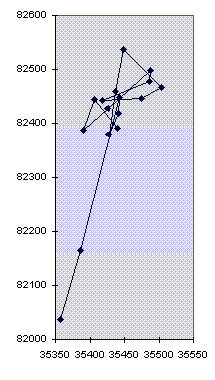
Getting fixes in these alpine conditions was no problem at all. Although the area is mountainous, you generally have a large area of sky visible and this meant that we nearly always had a full set of satellites visible. This means that you get altitude data as well as position data, although in general this was given as +/- 60m, (which is more like +/-120m allowing for SA). Also the waypoints and track log do not record altitude, so you have to write it down to get any record. I noticed that the position immediately after it got a fix could be way out (up to 1km), but after a couple of minutes it usually improved to be within the correct area. You can tell this once you have a few waypoints marked because you get a line on the map screen zooming in from way over to one side. (See Example, Figure 1, page 10)
Battery usage is an issue. The GPS 45 uses batteries quite fast. It takes 4 AA cells, and set of these alkalines will last about 10 hours use - more if it isn't continuous. For this sort of logging that means you can use a set up in a day or two, which is expensive and leaves you carrying an awful lot of batteries round with you. NiCads do work, but only give about 4 hours use. I got round this problem by using my FX5 as a power source. The GPS45 will take any input from 5 - 40V so any 5V or more battery pack should work. I stole the though-0the-headset charger bits off my charger, and attached them to a backplate hastily manufactured from a couple of layers of lilt-bottle plastic. This made a lightweight FX5 adapter, when soldered to the combined power/serial lead which already had a car ciggy-lighter connector and 9-pin D - makes a pretty strange-looking cable! The FX5 should power the unit for about 50 hours, although with external power at this voltage some units may be prone to shutting down. The GPS45 has a 'battery saver' mode which is appropriate for use where the unit is moving at constant velocity so it should be fine for entrance-logging. I did not know about this at the time, but it can give up to double the battery lifetime. When I find out how to enable it I'll give it a go.
We were unable to download all this data from the GPS whilst in Austria, despite soldering up a cable and peering at specsheets and software downloaded from the very useful GPS pages on the net, as the software/serial interface simply refused to play. This may be because the serial port on the GPS45 is an NMEA (marine instruments) standard, not the more familiar RS232, thus the voltage level is only 5V, somewhat below the 9-12V normally used on computers. Most serial interfaces will work anyway, but yours, like ours, may not. Either get a different serial card, or build a step-up interface - again, details of what you need are in the GPS net docs. This setback was inconvenient, but not serious as the track log was big enough to hold all the data we needed, so I could do the download and analysis on return to the UK.
Unfortunately, when I got back the GPS couldn't be found anywhere! I had noticed during packing of a huge pile of stuff into Julian's van that I hadn't specifically noticed it going in. Concerned, this being borrowed kit, I asked Julian, who assured me that he had seen me put it in earlier. 'Are you sure?', 'Yes, definitely', he said. Given that all our stuff had gone into this van, and I'd had it the day before in my rucksack, I had to assume he was right, and back to the UK we drove. However, once back, a great deal of checking showed no sign of it, and an increasing air of perplexed embarrassment settled. It must have fallen out of my rucksack somewhere on the last day, or been stolen from the campsite pile of rucksacks that night…. Then someone had the brilliant idea of leaving a message for one of the expedition members (the CSG's membership sec., Andy Atkinson, no less) who had gone on to the Imperial CCC expedition to Slovenia, and was returning via the campsite in Austria two weeks later. So a cryptic message about GPS units was left with the long-suffering Gasthof owner Karin, telling Andy to go and look for it on the mountain. He rang me at 6.30 one Saturday morning to get this bizarre message explained, and after the requisite grumble, set off up the mountain. Miraculously the GPS was sat quietly on the VD1 fixed point, the highest point of the route to our major cave, none the worse for it's two-week sojourn atop an Alp apart from an inexplicable cracked display. This was because four of us had left it there whilst chatting about glaciology on that last day, logging the VD1 position, and then had simply set off to go caving, forgetting about it entirely - ooops! So beware, that if distracted during the logging process, and if you are sufficiently dense, you may just leave the damn thing behind entirely! Garmin UK repaired the cracked screen for free, despite it being out of warranty, where it would normally cost 30 quid, and thus it finally got back to its owner.
This little setback dealt with I was finally able to download the track data using the simple, free Gardown7 utility, a no-frills bit of DOS software that simply generates a text file of data. You give a command like GARDOWN7 T S2 to download Track data on Serial port 2.This gives a text file with a header and then one line per track log point, like this:
T N49 37.7525 E006 12.2740 Fri Jul 12 22:51:49 1996
T N49 37.7441 E006 12.2804 Fri Jul 12 22:53:50 1996
T N49 37.7635 E006 12.3152 Fri Jul 12 22:55:51 1996
T N49 37.8224 E006 12.3338 Fri Jul 12 22:56:36 1996
T N49 38.1552 E006 12.8984 Fri Jul 12 22:58:36 1996
T N49 38.2060 E006 14.2361 Fri Jul 12 23:00:36 1996
T N49 38.3663 E006 15.8547 Fri Jul 12 23:02:38 1996
T N49 38.4481 E006 16.0234 Fri Jul 12 23:04:39 1996
This is: T for Track, Then the Northing and Easting (Lat. /Long) in Degrees and minutes, then Day, Month, Date, Time, Year.
I imported this data into Excel7 using the import text function to split this up into columns, and throw away the useless stuff like the T, N & E.. Having done this, I split the data up into sections by time, thus grouping all the logged points at one location together. At this point I realised a problem with my method. As the time is the only way you can tell which track log items were recorded where it is very important to turn the unit off between logging positions, otherwise you can't tell when you were standing still. It is possible to use the waypoint information that you have, as this is also timestamped, but basically be aware that if there are gaps in the datastream it is much easier to split up the sections. An alternative would be to record the GPS time (displayed by the GPS) on arrival and departure at a site, but you really do have to remember if keeping the unit on whilst wandering about. Keeping the unit on is useful because a) it's fun to play with and watch your little squiggle wander about the place, and b) you seem to get more accurate position data after the unit has had a fix for a few minutes.
There were 723 track log points, taken in 50 sections at 41 positions (some places were logged more than once to see what repeatability was like - (see Figure 2, page 15). For each section of logging the average position was calculated in X & Y. At this point I have to explain the complications of co-ordinate conversion. This is by far the biggest problem in using a GPS. Although the unit knows all about a whole host of co-ordinate systems and origins, the serial data downloaded is always in Lat./Long. format using the WGS84 spheroid. When you record positions they are likely to be in the locally useful co-ordinate system, and this is what you will need to plot positions on the map. In the UK this will be 'OSGB'. On an expedition you need to do a bit of research to find out what you should be using and how to do the necessary conversions. The OS publish a very useful couple of documents 'Transverse Mercator Projection - Constants, Formulae and Methods', and 'Conversion of Latitude and Longitude to/From National Grid'. I have photocopies of these if anyone needs them - they may now also be available on the net. These sums have been turned into a DOS program called 'CONVERT.EXE' (imaginative stuff!), and a RISCOS Basic program, both of which I also have.
The Austrian Grid system has proved to be something of a conundrum, and I still haven't reached a fully satisfactory answer. The maps themselves don't give any information about the Grid System in use, although they do have Lat./Long markings at the edges, but I have been given some information on the grid system in use, that Andy Waddington has discovered.
The co-ordinate system is called the Gauß + Krüger Landeskoordinatensystem, which is in fact a designed-to-confuse alternative name for Universal Transverse Mercator (UTM) and in this area is UTM zone 33. Within this system, there are a number of triangulation points surveyed purely for the purpose of locating caves: these are the Katastertriangulierungspunkte, or KT points. The X (or north) co-ordinate, when quoted in full, is actually the distance in metres north of the equator.
These Laser Rangefound points, use grid co-ordinates which can cause a great deal of confusion on several counts:
So we get points with co-ordinates like this ( prefix (52) for complete X co-ord.):
KT114_96 36670.37 83317.43 1903.97 Hinterer Schwarzmooskogel Trig point
Laser0 36386.56 82804.16 1815.45 Hilfstandpunkt (hillock N of 161)
Laser0_1 36093.56 82337.43 1782.35 Near 156
This is fine as far as it goes, but the GPS45 gives UTM and 'German' as different Grid systems. I believe 'German' to be the Gauß & Krüger referred to above as the readout is prefixed 'GK'. These two systems give similar, but not identical results, and neither of them is much like the values above, which is what we have the local fixed points marked in.
For example the point VD1 looks like this in the three systems:
UTM: 33T 0411506 5280946
G&K: 5411471 5283059
Laser: 36093 5282491
Fortunately all of these systems are a metric Grid,
so assuming that they are co-linear within the area in question,
then only an offset is required to convert from one to another.,
and the offsets from one system to another can be determined by
knowing one point in these two co-ordinate systems. More complexity
is added when you consider the Datum used. The above were done
using the Potsdam datum, but if you change it you will get slightly
different results. It is noticeable that the Northings all agree
to within 2.1km, but the Eastings are a bit more different. Ignoring
the 5million km figure then the UTM & G&K are the same
to within 35m, but the Austrian Laser points seem to be completely
unrelated.
A solution to all this confusion seemed to be the
software 'GEO2', written by Anton Helm at the university of Wien.
This software converts between Lat./Long and Gauß &
Krüger co-ordinates. In fact it is smarter than that and
can do any conversion between spheroidal co-ordinates (e.g. Lat./Long),
and any Grid System, given suitable parameters. It is rather 'UNIXy'
software, being a script-processing language where variables are
assigned to points and various operation can be done on these
variables to achieve conversions. I have to admit that I have
not fully investigated its results, but they seem to give yet
another set of different answers!
Given these discrepancies I have taken a rather pragmatic approach to doing the conversion from one co-ordinate system to another. I have assumed that over the 3km are that I am dealing with I can take Lat./Long. to be linearly mapped to the G&K grid, which means I simply have to find the offset and scale for the conversion. If I have two points for which I know both the Lat./Long. co-ordinates and the G&K co-ordinates then a simple interpolation will provide the conversion for all the other points. This will only give reasonable accuracy if the two known points are at opposite corners of the area in question. In fact Excel will let you give it a whole series of pairs of points and return the slope and intercept values of the best-fit line through them., so this is what I have done. To get 'correct' conversion from Lat./Long. to G&K, I have converted (rather laboriously) each averaged result for a point of interest into G&K using the GPS45. This is done by entering a waypoint in Lat./Long. mode, then changing the co-ordinate system to 'German', and looking at the waypoint again. This is rather a lot of button-pushing on the GPS, but it kept me entertained for a couple of long winter evenings over Xmas in the Pen-y-Pass youth hostel. Using all these pairs to get the slope & intercept values then comparing the calculated results with the GPS results, shows that the process gives results accurate to 15m across the area we are concerned with -good enough.
The final part of getting a set of cave entrances
that I can plot on the area map is the mysterious offset from
GPS-reported G&K co-ordinates to Austrian Laser Rangefound
co-ordinates. To do this I needed a laser point that I had reasonably
good GPS values for. I chose the one on Brauning Näse as
the GPS was left there for 8 readings, making it the most reliable
Laser point data I had. The problem with using a single point
for the offset is that any error in that GPS location is applied
to all the others too by being included in the offset from G&K
(Garmin) to G&K(Austrian Cavers). I still need to do further
investigation to determine the effects of this. The results could
be improved by taking multiple places where we have both G&K
(Austrian Cavers) co-ordinates and GPS locations and taking a
mean of the various offsets, or by doing better long-term GPS
locations (e.g. for a couple of days) at one of these points next
year. We have what should be a very good dataset for point VD1
(where the GPS was left accidentally), as it logged for 5.5 hours
before giving up due to flat batteries. Unfortunately this is
not an Austrian Laserpoint, although it is joined to one by a
surface survey. Using this point might well give better results,
but it depends how good the surface survey is.
So, after a great deal of head-scratching I have
a pair of columns on my spreadsheet giving co-ordinates in G&K
(Austrian Cavers) co-ordinates. It looks like this, showing the
actual data and (boxed) the averaged results: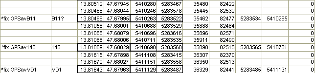 The
co-ordinate pairs are: decimalised Lat./Long., interpolated G&K,
offset 'Austrian' G&K, GPS calculated G&K (note X7Y reversed
on these, cos that's the way the GPS displays them).
The
co-ordinate pairs are: decimalised Lat./Long., interpolated G&K,
offset 'Austrian' G&K, GPS calculated G&K (note X7Y reversed
on these, cos that's the way the GPS displays them).
The easiest way to get this into Survex for plotting
is to put in a column that says *FIX <stationname> in front
of these columns, and putting an altitude value in at the end.
Then by hiding all the data lines, and all the columns except
the G&K (Austrian) ones, this section of the spreadsheet can
then be exported to a text file and processed directly. By including
the waypoints marked in the field (and given a similar treatment
to the track log data), it is possible to see whether the averaged
results are noticeably better than the waypoint results.
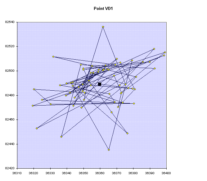
Here is typical example of the results:
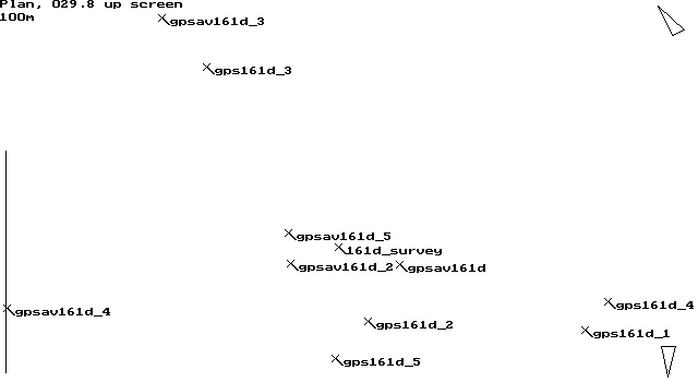 Figure
2, showing 5 fixes for entrance 161d,
and the 5 corresponding averaged positions.
Figure
2, showing 5 fixes for entrance 161d,
and the 5 corresponding averaged positions.
The averaged positions for locations 1,2 and 5 are all within about 25m of the surveyed point 161d, whereas the waypoints 1,2 & 5 are all 50-100m away. However the 3 & 4 averages are slightly further away than the corresponding waypoints. Location set 4 lasts for 25 minutes. After 20 minutes the position suddenly zooms off 500m to the E. It is this sort of odd behaviour that means a GPS reading alone can be thoroughly misleading. The bar on the left shows the 100m limit, and the readings are nearly all with in this, although not quite.
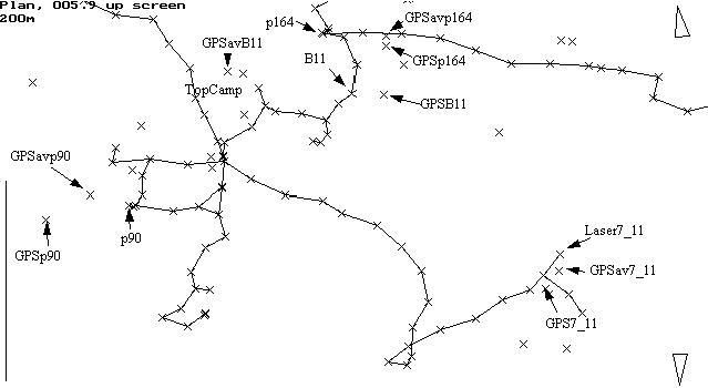 Figure 3, showing the area
of the plateau near top camp with surface surveys and GPS positions.
Figure 3, showing the area
of the plateau near top camp with surface surveys and GPS positions.
I have selected a number of locations, the corresponding
GPS waypoint, and the averaged track log data for it. As you can
see the averaged data is closer to the actual point than the waypoint
for Laser7_11, p90 and p164, although in the case of p164 there
is hardly any difference. These locations were averaged for only
about 20 minutes. The B11 data illustrates the importance of examining
the data graphically, and checking suspicious stuff. The point
marked GPSavB11 Was one where the track log had clearly rested
somewhere for a few minutes, and the timing (at the end f a day),
and known route that day suggested that it was B11, done on return
to top camp. This was what got written down (with a question mark
in the spreadsheet). After all the grid processing and displaying
the results in Survex I note that the waypoint at B11 is much
closer to the known position of the cave than the GPSavB11 location.
A quick check back to the track and waypoint data shows that the
waypoint was done two days later, and that there was a question
mark next to the GPSavB11 name. This all means that this isn't
B11 at all, but a short log at top camp whilst waiting for the
tea to brew. Again - record keeping is essential to avoid this
sort of mistake.
GPS is definitely useful in the field, but you need
to understand its limitations. To get the best out of it you need
to be diligent about how and when you record information so that
you can get the data out reliably afterwards, and you need to
understand about the co-ordinate system in use in the area, and
on the maps you have. Averaging is a useful technique, but can
be a rather hit-and-miss unless you can stay at a spot for at
least an hour, and for good results you need to be logging for
at least 4 hours, which means you need sufficient battery power,
and may not always be convenient in the field. Also beware turning
your GPS on, taking a waypoint immediately and walking off. -
it could be a long way out. If Differential GPS transmissions
are available in the area, then that will be much more effective
in giving accurate answers quickly - but of course it costs about
twice as much money, even if you don't have to pay for the data
as well as the receiver. As more of the far-flung caves in our
area are surveyed-to, we will be able see how it compares in accuracy
to very long surface surveys. And some time in the next ten years
the US should turn off SA which will make life significantly easier
for this sort of work.