EVENTS
Problems to be aware of when using radiolocation
How accurate is Radioloaction - Practice - Stuart France
Radioloaction experiment at KMC
Enhanced LRUD Recording - Andy Atkinson
Further discussion of blunder prediction issues
Onstation, Rotater, Compass Home Companion, Survex
Those of you who were at the BCRA conference will hopefully have noticed the Special Interest Group Stand we set up this year. The Surveying Group had a significant presence, with a satisfying pile of computers, largely courtesy of Nick Williams. I hope that a few of you reading now are new members who signed up there.
I had the bright idea of giving away software to anyone who wanted it, and even brought a box of floppies, as most people don't think to take such things with them to the conference. This was very popular, but had the disadvantage that I spend a large portion of the weekend formatting and copying floppies. Next year I will take some preformatted ones at least! A large number of copies of Survex &Compass were taken away, and I haven't had any complaints, so I assume that people are finding them useful.
17-19 May 1996 in the Peak District. More details in the Newssheet, or contact Mike Bedford. On the surveying front at this meeting we will be holding a discussion forum on LRUD data recording techniques. The current standard causes significant problems when interpreted by a computer to include walls with the centreline. Andy Atkinson's article in this issue is one suggestion for recording a little more data that would go a long way to improving the survey software's output. Obviously it is important for both surveyors and software authors to understand each other's requirements and limitations, and thus to work out what is the best compromise in terms of data recorded and results produced. I would invite anyone who has an interest in this area to turn up to the discussion. Some more practical surveying experiments are also likely, such as more on radiolocation, and Suunto person-to-person variability.
This is 24th Feb 1996 at the University of Staffordshire. This has been largely the preserve of the rocks & bugs people for some time now (like Cave Science), so Dave and I are doing our bit to raise the profile of the rest of cave science. I will be giving a paper on 'Cave surveying software - the state of the Art'. This will be a broad overview of what is now available in both general terms (facilities) and specifics (particular pieces of software). I will also be looking at the forthcoming developments in software, such as blunder detection, final survey production, GIS in caves, etc. The results of the Field meeting discussion on data recording will also feature.
This annual award is made to reward outstanding effort in Surveying in the UK. It consists of an old miners dial compass in engraved presentation box. Which the winner get to stick on their mantlepiece for a year. This year it was won by Chelsea Speleological Society for their huge efforts on the Grade 5 Ogof Draenen Survey, even though it isn't quite finished! Apparently this publication came a close second.
Wookey
I have just got an up to date price list for from the UK Suunto distributor Viking Optical. They seem very fussy about dealing direct with the 'public' so to get these deals we need to go through my company. Anyone interested in ordering anything please contact me at the editorial address. Cheque with order please. These prices include VAT. Add £3 for postage & hassle. If you think you need registered post then add another £2.
| RRP | ||
| KB-14/360 | £65 | (£99.95) |
| KB-14/360 (Drain holes) | £74 | (£114.00) |
| KB-14/360R | £65 | (£99.95) |
| KB-14/360RT | £85 | (£129.95) |
| KB-14/360B | £91 | (139.50) |
| PM-5/360PC | £83 | (£128.00) |
| PM-5/360PC (Drain holes) | £93 | (£142.00) |
| PM-5/360PCT | £98 | (£150.00) |
| PM-5/360PCB | £103 | (£159.00) |
| TWIN 360PC (comp + clino) | £143 | (£219.95) |
| Rubber cover (Black or Yellow) | £5.50 | (£8.50) |
The more obscure variations are also available, as is the rest of Suunto's range. Contact me if you need anything else.
Tim Long, Morgannwg Caving Club
I thought that users of Survex might be interested in the way I organise my data files. I'd like to hear from anyone who has any other strategies, for whatever reason.
I arrange my data so that I have one passage or passage segment per file, to keep the survey in manageable chunks. I have adopted an object orientated approach in that each file "exports" information about where it joins other passages. To use an example from the Ogof Draenen survey, I have two passages recently discovered by Oxford University Caving Club, called "St. Giles" and "Lamb Passage". In the Lamb Passage survey...
*Begin Lamb
*Equate 1 StGiles	[creates a station called Lamb.StGiles,
                                          equivalent to Lamb.1]
*End Lamb
This does not specify exactly where in St. Giles the passage joins; it merely describes that it joins St. Giles somewhere. The other half of the information is contained in the St. Giles data:
*Begin StGiles
*Equate 3 Lamb	[creates station StGiles.Lamb equivalent to StGiles.3]
*End
The two pieces of information are brought together by a third file, links.svx, that "glues" all the passages together. For the above connection, it contains the line:
*Equate StGiles.Lamb Lamb.StGiles
Finally, my "master survey" file, draenen.svx, is along the lines of:
*Include Links
*Include StGiles
*Include Lamb
The advantages of this method are not obvious until you consider that there are two surveys in progress for Ogof Draenen. I have recently replaced the entire Gilwern Passage grade 2 survey data with grade 5 data. The Grade 5 survey has different station names, but by exporting the connections from the grade 5 file, there is no need to change anything else. I can chop and change between grade 2 and grade 5 just by including the appropriate file. The same links.svx file works for both cases. I keep data in separate subdirectories, because I have both grade 2 and grade 5 surveys for some passages. Say a grade 5 survey of Lamb Passages comes along to replace the grade 2 data. My draenen.svx file becomes:
*Include Links
*Include Grade2\StGiles
*Include Grade5\Lamb
I can use the grade 2 or the grade 5 version of lamb passage just by changing the *Include. Nothing else needs to change.
The situation of having two surveys might seem a
bit bizarre, but Morgannwg Caving Club has discovered over 27
km of passages in under seven months! The explorers set a strict
rule very early on that all leads were to be surveyed to BCRA
grade 2 (grade 3 but clino not always used) as they were explored.
The data was quickly collected and fed into Survex, allowing us
to plan the following week's exploration. Meanwhile, a much more
detailed grade 5 survey was started by other cavers. The grade
2 survey is kept accurate almost up to the minute with the latest
discoveries; it is our "pushing survey" and gives us
our official cave length. As grade 5 data becomes available, it
will be incorporated into the pushing survey, giving a better
idea of vertical relationships between passages, adding more detail
and making the survey much more accurate. When complete, the grade
5 data will form the basis (centre line plot) of a properly drawn
up and annotated survey. The two different surveys also serve
as a very useful cross-check and a few gross errors have been
highlighted by overlaying the two surveys.
Daniel Gebauer
Readers of Compass Points know how to light a Suunto with the help of a module gunged with silicon sealant to the surface of the instrument without modifying the instrument itself (GEBAUER, CP2: p3; WOOKEY, CP7: pp7-9). The light emitting assemblage is controllable (can be switched on/off), consists of four to five cheap pieces (LED, battery, switch, odd bits of wiring), and is interconnected by five to eight soldering points. This module appears to be quite simple but Zen masters ask to clap with a single hand. Unexpectedly the complexity of a controllable lighting module for Suunto instruments can be drastically reduced to LED plus battery soldered together with a single soldering point.
No extra switch is necessary when you use the LED-legs. One leg of the LED is soldered to the battery which touches the metal body of the Suunto. The second leg is allowed to have some room to move and will touch the Suunto body when the silicon sealant cover is squeezed.
Such a crude construction was expected to fail either immediately or at least pretty soon. Please don't blame me, but it has survived a fortnight of Austria's CRUW-type (cold, rough, ugly & wet) caves and another month of mapping PAHW-rivercaves (pleasant, amiable, humid & warm) in Tanzania. It still works and I will take it to Meghalaya next week.
A few precautions I reckon to be advisable: Improve ease of contact by increasing the surface of the LED's switching leg; By rubbing the Suunto body's surface with an old style ink eraser; and by applying conductive grease. Concerning the colour of the light red is by far the best choice. A red LED consumes least electric power, is easiest distinguished by human eyesight in darkness, and causes least disturbance to adaptation. A cylinder shaped LED is improved by grinding one side flat: The sanded surface diffuses the light and the LED itself comes closer to the point where it is needed. A tiny scrap of aluminium foil which covers the far side of the LED functions as a reflector. Keep the reflector small to allow access for foreign light.
The configuration of the VHS Lighting Module requires some fumbling to bend it to a snug alignment with the Suunto. The battery, for example, must needs lie flat on the body, the LED should almost touch the transparent capsule close to the spot where the illumination is most effective. To be on the safe side, the free leg of the LED could be guarded by a small strip of some insulation which, however, should not be allowed to disturb the snug alignment of the battery. The far end of the LED's free leg runs around the edge of the Suunto's body at a distance of about half a millimetre. Having adjusted the bending angles of the VHS Lighting Module, a wee wee tiny little smack of conductive grease is attached to the centre of the battery's back. Then the module is preliminarily gunged with two or three limited smears of clear silicone sealant. This is the stage where the last corrections are possible. Leave the almost completed lighting rig alone for at least several hours, better a day. Take care to cover the switching LED-leg with a bit of paper or tape to prevent silicone sealant to enter the gap between leg and body which is necessary to (dis-) connect the current.
by David Gibson
The accuracy of cave surveys, and the treatment of measurement errors has been discussed many times. Often surveys are "corrected" by means of radio-location, but the question of the accuracy of radio-location has not been widely debated.
Radio-location using an induction loop is, by now, a standard procedure. I will not explain it in detail here. You should refer to Dick Glover's (1976) definitive description of the technique in Surveying Caves or, for a more recent discussion - which includes a reprint of the circuit of the France/Mackin radio-locator - to Bedford, (1993).
This article will identify some of the sources of measurement error, but it will not attempt to quantify them. In that sense, it will not answer the question posed in the title. The intention is to bring the sources of error to the notice of cave surveyors and to encourage further discussion and reporting. Theoretical and practical evaluation of errors may be a topic for future articles.
Some useful practical work has already been done - mainly, it would seem, by cavers in the United States - but little has been widely published in the UK. A trawl through the index to BCRA Transactions showed that the subject has hardly appeared. However, Brooks & Ellis (1956) shows that attempts in using radio-location for verifying cave surveys go back at least forty years.
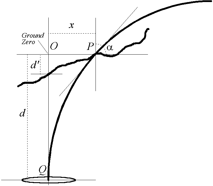
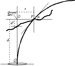
Essentially, a horizontal transmitter loop is placed underground and the point on the surface immediately above this is located with a receiver loop.
At this "ground zero" point the magnetic field lines from the transmitter are vertical so a vertical loop (i.e. with its axis horizontal) will pick up no signal because the field lines do not "cut" the loop. The ground zero point is confirmed by holding the loop vertical, spinning it about a vertical axis, and confirming that there is no orientation where a signal can be detected.
To locate ground zero from another location the vertical receiver loop is rotated to give the direction of maximum signal, and a bearing taken. A series of at least three widely spaced bearings will intersect exactly, if you are lucky, or else they will give you a "polygon of confusion" inside which the ground zero occurs.
The depth of the underground point can be determined in two ways. The easiest method (with the right equipment) is, perhaps, to measure the flux density (say B0) at ground zero and to compare this with the signal (B1) a short distance (y) above this. Using the ratio of these readings provides a convenient way of calculating the depth, d, without needing to know the transmitter power or absolute gain of the receiver. We use the inverse cube law, to get
 (1)
(1)The more common method of depth determination is to measure the angle of the field lines. Away from ground-zero the magnetic field lines are not vertical. By measuring the angle of the field to the ground (), and knowing the distance to the ground-zero point (x), we can calculate the depth of the transmitter (d) - Figure 1.
This method relies on the field lines obeying the parametric equations for a traditional "bar magnet". The formula is
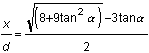 (2)
(2)A convenient technique for depth estimation is to find the distance x at which the field lines lie at 45° to the ground. The formula then tells us that x/d 0.56, so the depth is approximately twice the distance x. Another technique would be to find the distance x at which the field lines were at 18.4°, for which x/d = 1.
Clearly there is plenty of scope for errors of measurement to have an effect. Most of the sources of error affect the depth measurement more than they affect the location of ground-zero. The accuracy of a position fix also depends, of course, on the accuracy of the surface survey.
Ideally we would take several bearings in order to locate ground-zero as accurately as possible. Then, we would make field angle measurements at varying distances, plot them on a graph, obtain a best-fit curve and use this to determine depth. In practice we might only make one or two measurements but, if this is the case, the confidence of the result must be called into question - as it would with any problem in metrology.2
Glover (1976) demonstrates various graphical methods of converting and x into depth. His graphs demonstrate how small errors in reading can lead to large errors in depth. If = 80°, for example, then a 1° increase in corresponds to an decrease in x/d from 0.117 to 0.105, which is 10%. At = 45° the change is only 2.5%. Mixon & Blenz (1964) also discussed angular errors in their paper.
Measuring the angle of the field lines on the surface requires us to accurately sight on the ground-zero point. As we adjust for the null position by tilting the receiver loop, we must ensure that it remains pointing towards ground-zero. Obtaining an accurate null, and accurately measuring the angle of the loop are crucial aspects of the technique.
Obtaining a good null is not always easy. There is a secondary field effect (see later) which makes it increasingly difficult to get a deep null as the angle of the field lines, , decreases. Depth measurements should, ideally, be made with from 40° to 50°.
The underground transmitter must be set up as accurately horizontal as possible. If the transmitter is only levelled to 5° the axial field line will be displaced by 8.7% of the depth (i.e. tan 5°) The field line which happens to be vertical as it leaves the ground will not be displaced quite as much as this but clearly there is still a large error.
Significantly, if the transmitter loop is not completely horizontal there will not be a field line which remains vertical as it leaves the ground. This could cause the null to be less sharp since there will always be some lines cutting the loop. In practice we can do better than 5°, but a spirit level is essential, as is a neatly wound induction loop.
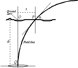
If the ground is sloping then equation 2 can still apply, but x must be the true horizontal distance to ground zero, and d is measured from the altitude of the field point. See Figure 2. Distance d must be determined by surveying.
Clearly the terrain can be a source of measurement error. In addition to the obvious "sighting" errors it is possible to detect a false ground zero, especially if the estimation of the surface location is tenuous to begin with. (Reid, 1990).
There is another source of error, potentially far more serious than the measurement errors described above. It is caused by the magnetic field lines departing from the supposed "bar magnet" shape. There are several reasons for this.
i) The receiver loop may be too close to the transmitter.
Unless it is far enough away for the transmitter to look like a point source, the field lines will be distorted. In practice this means around five diameters. This will not normally be a problem but, if you are in the habit of using a 2m transmitter loop, then you must be at a depth of at least 10m to get an accurate reading. With a smaller loop you could probably get a reasonable result closer than five diameters because you could tolerate a larger margin of error.
Not only are the field lines distorted in the immediate vicinity of the transmitter loop, but the familiar inverse cube law breaks down too, so equation 1 cannot be used for depth estimation.
It is possible to derive an expression for the field from a "finite" loop, but it is complicated. Mixon & Blenz quoted a previous author, but you will also find the method in a modern text book on e/m fields.
ii) The field lines will be distorted by magnetic rocks.
The distortion of field lines is exploited by geophysicists and archaeologists, who use magnetometers as surveying tools. There is not a lot you can do except to avoid using radio-location in areas where there is a lot of mineralisation. Unless, of course, you want to develop a cave detection technique based on this phenomenon. Unfortunately, unless you prepare a control grid of readings which are correlated with an accurate compass & clinometer survey, you will not know how much this problem affects you.
iii) Distortion by conductive rock - the "phase" problem
The absence of magnetic rocks and minerals does not solve the problem because conductive rock can also distort the field lines. Again, this effect is well-known to geophysicists and archaeologists who use a surveying tool called a magnetic gradiometer which induces a field in the rock and measures its distortion.
The effect of a magnetic field passing through conductive rock is to introduce eddy currents. This generates a so-called secondary magnetic field. This field is out of phase with the primary field. It leads to a condition known as elliptical polarisation and prevents us from obtaining a full "null" condition. The problem was discussed by Drummond (1987a) and Gibson (1993a). The problem is worse at larger distances. Just as with the previous problem, the phenomenon is of use to geophysicists, who can use it to measure conductivity by a non-contact means. (Pease, 1991, 1995).
iv) The "Transition Zone" problem
The field from an induction loop can be divided in to two regions. The near-field (or induction field) predominates at distances less than /2 ( is wavelength). The far-field (or radiation field) predominates at distances greater than this. The two fields have very different properties. For a large distance either side of /2 there is a transition zone where the field changes from the induction "bar magnet" shape to concentric circles which do not intersect the origin. The inference is obvious - if we are in the transition zone the field lines will not behave as predicted above.
The "transition zone" and "phase" problems can be discussed together as a "polarisation" problem. One or other of the effects have been observed by a number of people, though they are not always attributed to the correct causes3.
The transition zone is centred on /2 and you might expect this to be very large at the low frequencies we are using. However, the crucially important point is that the wavelength in the rock is much less than this. The transition zone moves inward to (and the wavelength to 2) where is the skin depth, given by
 (3)
(3)Skin depth is discussed by Gibson (1993a, b). It can vary from a metre or two to several hundred metres, for the range of frequencies and rock types we would encounter. It is quite conceivable that a radio-location beacon could be operating at depths comparable with the skin depth and where the transition zone effects would be significant. At this distance, secondary fields would also be significant. Interestingly, the optimum depth for communications (as opposed to radio-location) may be around three skin depths (Gibson, 1993b, 1994)
These effects have been analysed by many people over the years, often in dense mathematical terms in journals of physics. Steven Shope (1991) has summarised some of this work and he has written a computer program to show how the direction of the field lines at the surface depends on the skin depth. One of these graphs was reproduced by Bedford (1993).
Shope's graphs are extremely important. They show that in some circumstances the result given by (2) can be wildly in error. I will be analysing this source of error in a future article (either here or in the Cave Radio Group journal). Suffice to say that if you are interested in the accuracy of radio-location you should read Shope and be well aware of the significance of his results.
It is worth pointing out that it is not only the field angle which departs from simple "bar magnet" theory. The 1/D3 rule for flux density also breaks down in the transition zone, so equation 1 cannot be used for depth determination either.
The measurement problems can be quantified and used to make an estimate of the accuracy, which could easily be 5-10% for depth, and several metres for ground zero.
The polarisation problems are less easy to quantify. Depth determination starts to fail if a good null cannot be obtained, eventually failing completely. In these circumstances a ground-zero location can often still be performed. This only starts to fail if the rock is anisotropic, or the ground is inhomogenous in some way (e.g. close to a fault-line or chamber).
The problem of the transition zone is lessened considerably by using a very low frequency, because the zone is further away, and because the secondary fields have a lower magnitude. The France/Mackin beacon operates at 874Hz; several US designs operate at 3496Hz. Radio-location at these frequencies is likely to be more successful than if it is done using carrier-based speech systems; common frequencies for which are around 27, 87, 115 and 185kHz. See Bedford (1994).
I have dealt here with the conventional "caving" method of using field angle on the surface to locate an underground transmitter which must be horizontal. There is a commercial mining application where the locator has to find a small transmitter in unknown orientation, in conductive coal measures, from underground, without access to the ground surface. The algorithms to do this are extremely complicated and would make an interesting caving study.
Ian Drummond (1987b) described some experiments which he, and others, did in Lechuguilla Cave in New Mexico. Amongst them was a series of radio-locations along a passage at a depth of up to 210m. The purpose was to see if the magnetic field was well behaved, and if it diverged symmetrically from the null point. Plotting the data (and re-surveying part of the cave to check for errors) showed that the field was badly distorted in one area. This was attributed to mineralisation of a particular cross-rift.
The experiments confirmed the wisdom of performing a series of locations to provide a control grid for a survey, rather than relying on one single point at the far end of the cave to check the survey.
Drummond also found that the sharpness of the nulls depended on the orientation of the antenna. The precision of the location on the surface was much better along the passage than at right angles to it. This may well be a secondary field effect, but Drummond has noticed a similar effect on other occasions and suggests (quoted in Gibson 1993b) that it could be an anisotropic characteristic of the rock.
Another observation arising from experiments in several countries, is that the UK is particularly badly off for rock conductivity and background interference. The inferences are that polarisation effects are likely to be worse, and that nulls are likely to be less sharp. At Cave Radio Group field meetings we have demonstrated that radios which penetrate well in the US do not work so well in the UK. A narrow-band receiver using a phase-locked-loop could make a significant improvement here.
Radio-location works best at very low frequencies (below a few kHz) and over distances which are short compared to the skin depth, but large compared to the size of the loop. Its accuracy is affected not only by measurement error, but by factors which are difficult to predict, such as distortion of the field lines.
Statements such as "we fixed the position by radio-location" suggest a misplaced confidence that the technique has an unfailing accuracy. Users must understand how to minimise the measurement errors, and how to deal with uneven terrain.
This article was intended to make users aware of the possible inaccuracies of radio-location, rather than to ascribe figures to the sources of error. Occasional tests of accuracy have been made but not widely reported. The list of references contains material specifically oriented towards cavers, but the techniques are well-covered in geophysics and electromagnetics textbooks, as well as in various caving club publications.
I would like to thank those people who discussed an early draft of this article with me - Olly Betts, Bryan Ellis, Stuart France and Wookey. And especially Ian Drummond who made many useful comments and reminded me of the work done by Bob Buecher, Frank Reid and others.
Bedford, Mike (1993), An Introduction to Radio-Location, JCREG 14, Dec. 1993, pp16-18, 14
Bedford, Mike (1994), A Directory of Cave Radio Designs, JCREG 18, Dec. 1994, pp3-4
Brooks, N,. & Ellis, B (1956), An Independent Check on the Survey of OFD, South Wales Caving Club Newsletter 16
Drummond, Ian (1987a), Magnetic Moments #5: The Phase Problem, Speleonics 7, Spr. 87, pp11-12
Drummond, Ian (1987b), A Cave Radio in the Field - Summer 87, Speleonics 9, Winter 87, pp7-8
Gibson, David (1993a), An Introduction to Cave Radio, JCREG 12, June 1993, pp24-26
Gibson, David (1993b), Penetration of Magnetic Fields Underground - Part 3, JCREG 14, Dec 1993, pp21-25
Gibson, David (1994), Penetration of Magnetic Fields Underground - Appendices, JCREG 15, March 1994, pp19-21
Glover, R.R (1973), Cave Depth Measurement by Magnetic Induction, Lancaster Uni. Speleo. Soc. Journal 1(3), pp66-72, Summer 1973
Glover, R.R (1976), Cave Surveying by Magnetic Induction, Surveying Caves (ed. B. Ellis), BCRA
Mixon, W. & Blenz, R. (1964), Locating an Underground Transmitter by Surface Measurements, The Windy City Speleonews, 4(6) pp47-53. [also: reprint in Speleo Digest 1964]
Pease, Brian (1991), Measuring Ground Conductivity with a Cave Radio, Speleonics 16, May 1991, pp4-6
Pease, Brian (1995), Letters, JCREG 21, Sept. 95, p29
Reid, Frank (1990), False Center Found in Unusual Location, Speleonics 15, Oct. 1990, p15
Shope, Steven (1991), A Theoretical Model of Radio Location, NSS Bulletin Vol. 53 No 2, Dec 1991, pp83-88
JCREG is the Journal of the BCRA's Cave Radio & Electronics Group. Speleonics is the newsletter of the Communications and Electronics section of the NSS (National Speleological Association, USA). Copyright ©David Gibson, 1995
Stuart France
The loop-closure error in a grade five survey of the Kingsdale Master Cave (KMC) entrance series using conventional surveying and radiolocation plumbs was small on an experiment at the recent BCRA CREG field meeting.
KMC is a useful site for cave radio experiments, being close to the road, easy underground terrain, and relatively level cave going into a hillside rising steeply to the west side of Kingsdale. It would be useful to have a few surface fixes for passages at increasing depth to test equipment and techniques. The October 1995 BCRA CREG field meeting set out to survey these using the France/Mackin 874Hz radiolocation rig [1]. Four underground sites were selected at estimated depths of approximately 20, 50, 70 and 90 metres based on the ULSA cave survey [2] and 1:25,000 OS map contours.
A BCRA grade 5 centre-line survey was made by Stuart
France and Margaret Bedford from the entrance, taking the centre
of the bottom rim of the surface end of the oil drum as [69885,77400,267]
from inspection of the ULSA survey. The coordinates of the four
underground locations, marked nearby with postage-stamp sized
blue paint spots, were computed as follows:
| Location | Coordinates |
| Largest flat-topped boulder in left-hand alcove just before first deep water | [69850, 77411, 266] |
| Floor of passage below step down in roof looking into the Toyland/KMC junction | [69805, 77458, 263] |
| Smoothest floor on right just before line of bolts looking at ladder pitch head | [69820, 77675, 258] |
| Flat sand bank just before flat-out section some 5m south of waterfall up to Toyland | [69719, 77430, 264] |
All four sites except the pitch head agree with coordinates derived from the ULSA survey to two metres or less. This 17' pitch, as shown on the ULSA survey which gives no spot heights, is at [69830,77693] giving a large discrepancy of [10,18] yet to be resolved.
The first two sites were radiolocated on the surface using an 18" square rigid wooden antenna. Underground was a collapsible ribbon cable square antenna, also of side 18", held taut on a cross-shaped former made from two sections of oval PVC conduit passed through a central hub made of PVC wastepipe and levelled with a 6" spirit level. Vertical and 45-degree tilt on the surface antenna were measured with a 6" wooden protractor and brass strip pendulum arrangement that was clamped to the side of the square antenna. The underground group did not find their antenna easy to level perfectly and could see advantages (except in terms of portability) in having a rigid wooden-framed antenna underground too.
The approximate ground zero was located by intersection of lines of null signal observed some 10-20 metres back. Ground zero was fixed exactly using the antenna in vertical orientation whilst applying a full 360-degree rotation to find the best all-round null in the vicinity of the estimated ground zero, as described in [1]. Those people who tried this for themselves commented on how sharp the nulls were, both in the rough estimate and also the 360-degree rotation. The surface fix was linked into the underground survey with compass, clinometer and tape, taking a line from the oil drum up the hillside. The depth was determined by backing off from ground zero along the horizontal and measuring the separation from ground zero at a point where a null was obtained with a 45-degree tilt away from the fix (the depth is 1.77 times this horizontal separation). This measurement was done twice, either side of ground zero on the horizontal, and the average value taken. The results for the first two stations shown above were:
[69849.7, 77411.3, 265.7] | [69850.2, 77410.0, 283.0] | ||
[69804.8, 77458.0, 263.2] | [69805.5, 77456.4, 307.5] |
These results show errors of 0.3m (2%) and 2.7m (6%) respectively for the depth determination. The misclosures given as a percentage of the length of the loop are 1.28% and 1.07% respectively. The surface positions have been well marked using rocks with large blue paint spots. The remaining two underground stations will be radiolocated at a later date when it is also intended to install fixed wooden stakes to assist future experiments.
References
[1] France S & Mackin R (1991), Making a simple radiolocation device, Caves & Caving No.52
[2] Brook A & Brook D (1967), ULSA West Kingsdale cave survey.
Andy Atkinson
A number of survey software packages now let you include LRUD (Left Right Up Down) passage dimensions in some form or other and will produce a plot using this information. All of these, with the exception of Toporobot, are simplistic in their approach, and if you have seen the output you will recognise the rather odd-looking characteristic shapes that occur. There are good reasons why this is so. The conventions that surveyors use when recording the data, such as 'in the direction of the survey', and 'across the passage' are not very easily defined in computing terms. Also the fact that LRUDs are typically taken at stations, and stations are often at junctions causes problems as junctions tend to be atypical, rather than typical, of the passage. There are a whole host of other things like what to do when a value is not given, a question mark is entered, and at the ends of passages. If zero is assumed at an omitted reading then a pinch-point occurs in the walls at that station - not really the desired effect.
We have been examining the details of this process with a view to implementing something in Survex, and generationg a proper 3D model of the complex Kaninchenhohle. It quickly became clear that as well as the programming difficulties there were significant problems in terms of the data that was actually collected. Obviously a set of 4 numbers conveys much less information than a sketch. Unfortunately a sketch is inherently 2-dimensional, and thus is not very helpful when trying to construct a 3D model. So the question becomes - what is the least information that needs to be recorded in order to construct a useful 3D model? Obviously the answer depends on what you want to use the finished model for, and the usual constraints on surveying manpower, time & conditions.
Andy Atkinson took a look at the specific area of improving the information contained in the LRUD data without dramatically increasing the time it took to record, or the complexity beyond the point which surveyors would stand (where relatively inexperienced Cambridge Cavers in Austria's horrible caves have a particularly low tolerance of such things). Obviously improvements of this nature are no use if surveyors think they are too much extra work. Here he presents his second iteration of the idea for comment.
The computing aspects of LRUD interpretation and
the broader issues of wall modelling need articles of their own
to explore. These will be in future issues.
The suggested format is an extension of the now standard LRUD, with a 5th column -'E' for Extension - which is used in some cases. One obvious improvement is a notation for allowing more than one value to be given in the same direction. This particularly useful in traversable rift where you really want to indicate the distance to both the actual and apparent floors, or sometimes in a wide bedding where only the centre part is person-sized. There are many possibly notations, all prone to confusion, or not completely general.
 | L & R are defined as the bisector of the legs. For the last station they are perpendicular to the last leg. ~ is used to indicate estimated distances (very useful to know which numbers may be suspect when drawing up) | ||||||
 | (220) | Where L or R in standard direction is unhelpful, irrelevant or meaningless another direction is given. The approximate bearing is given in the comments field. | |||||
Pn | P(n) |
P(n) | P(n) | (NE)(160)(260) | For pitches give NSEW instead of LRUD. Where NSEW is not appropriate (e.g. axes of elliptical shaft lie in another orientation) then use bracket notation to give bearings | ||
 | At a Junction the value that would otherwise disappear down the joining passage is given as where the wall would have been if the joining passage was not there. | ||||||
 | When a survey ends at a junction the L & R values for the surveyed passage as if it continued are given. Also given is the 'Extension'. The distance that the survey leg would need to be continued to meet the wall. | ||||||
 | At a point where a passage meets a pitch The extension is given to the far wall and the roof or floor (roof in the example) is given using the Junction notation. | ||||||
 | For a perimeter survey use C (for Chamber) in either the L (anticlockwise survey) or R (clockwise) column. Readings are on bisectors of legs | ||||||
  | C Cn | C Cn | n n | n n | n n | For a radial survey the centre point is given like this Then the other give the Extension value to the wall, as well as U & D In more complex areas L & R values can also be given if they are significant | |
 | For more complicated bits of the cave the notations given can be combined to fit the need |
This quarter we have three completely new (to me at least) pieces of software. The Compass Home Companion, OnStation, and Rotator. There is also a maintenance release of Survex. And yet another Compass release, but this mag is full again, so you'll have to wait for details of that.
Paul Burger
COMPASS for Windows has a new third party product called "Compass Home Companion." It is the first product written by another author to support COMPASS. Compass Home Companion is a Windows based utility that compiles cave statistics not provided by other Compass programs. The program calculates survey length by year, number of surveys per year, length by person, number of surveys by person. It also does two different types of circular rose diagrams: length and frequency. The yearly results are displayed as beautifully colored bar charts. The rose diagrams are displayed as coloured circular graphic diagrams. There is extensive Windows style context sensitive help.
"Compass Home Companion" is currently
available as freeware. (Later versions will distributed shareware.)
It is on the US FTP site.
email: paburger@nhpsun.cr.usgs.gov
This is written by Taco van Ieperen, a Canadian. It has been designed from the ground up as a 32bit Windows application, and thus will only run on Windows95, or Windows 3.1x with the very latest version of Win32s (v1.30). I have only had time to have a quick play with the software but it looks promising. The interface is very nice with thumbwheels for movement & rotation, and plenty of options - colouring by depth, survey & year, 3d coloured glasses view, perspective view etc. Surface data can be included as a grid.
It also has a very general input facility which will read any text file containing lines of 'From To Tape Compass Clino L R U D'- type data, as well as specific ones for spreadsheet data and SMAPS data. A useful looking survey-tree editor is provided to let you allocate surveys to groups and select them for editing in spreadsheet-like tables. There are also lots of tabbed dialog boxes for setting information about the survey. The main thing that is missing is any loop closure. This bit is being written by someone else and so is not yet ready.
All in all this looks pretty good for version 1.0, and seems generally stable. I don't know how much complexity it can handle yet - look out for a review when I get a chance.
Mac Cavers! I am spreading the word about an AMAZING piece of software that does wonderful cave stuff! (Sorry I am getting so excited, but I hate complicated, slow, memory-hog programs, with crummy interfaces, and this one ISN'T. It is very MAC, simple to use, no need for manuals, etc.)
It is called ROTATER. As described by the programmer: "This is a program that reads a set of 3-dimensional points and lines and plots them in a window. The image can then be rotated with the mouse in real time." Boy, is that an understatement. Cavers already have a set of 3D points from crunching their survey data, so you just take those X,Y,Z coordinates and add a fourth column of single digit numbers to designate where to put a point and where to draw a line, and your data set is ready. Save it as a text file, and run it in Rotater. WOW! grab it with the mouse as if touching the outside surface of a ball with the cave inside, and rotate away! What was moments before a 2D line is now moving 3D in space. Also, the lines closest to the front are lighter than in the back as if front-lit which helps the effect even more.
I wrote a little macro in Excel to figure the coordinates for a bounding cube around the cave in a different color. When the cave and the bounding cube rotate together it is even more impressive. I used Rotater to view a cave with lots of vertical passage and a confusing overlapping maze area and I could suddenly visualize what was never clear before.
If you have a Mac, you gotta see this. I downloaded it from, http://raru.adelaide.edu.au/rotater/.
Software written by Craig Kloeden
Email: craig@raru.adelaide.edu.au
Version 0.62 includes a new option in PrintPCL to
deal with older PCL printers, and a fix for a bug in PrintDM.
This was the version available at the BCRA conference. A proper
new release with a pile of small-but-handy improvements to Caverot
and the Printer drivers should be out fairly shortly after this
issue of CP.